The Complete Guide to Modeling in Data Hub
Estimated reading time: 3 hrs.
Welcome
Welcome to this complete guide to modeling in Data Hub. The intent of this article is to provide you with the knowledge required to build out complete data models. While this is a lengthy article, it serves as an alternative learning path to the Data Hub modeling training course. That is, this article covers the same content as the Basics, Intermediate, and Advanced modeling modules taken together. Because this article covers the equivalent of three training modules, it does not go as deep into individual features. Instead, it assumes you will make use of the online documentation as required. At the end of this article is a list of next steps that you may consider to bed in the knowledge you gain.
Basic concepts
Let’s first introduce a few data concepts. We will start right at the beginning. A database is a data store that holds tables of information. Tables have rows and columns, and tables may relate to each other. For example, a Sales Order Lines table may relate to the Sales Order table.
A data model is a high-level plan of a database’s tables, table columns, and how the tables relate. A well-designed data model captures all tables, columns, and relationships relevant to your business. It should use friendly names, use your business terminology, and ultimately, it should make report design a simple matter of drag-and-drop. You don’t query a data model directly. Instead, a database is built to conform to your data model, and you query that database. Data Hub can generate two different types of database for this purpose, a data warehouse, and a semantic layer.
A data warehouse (or simply “warehouse”) is a database designed specifically for reporting or analytics (charts and dashboards). While your data may already be in a database, that database is likely to be designed for the operation of the source application. Such a “source” database rarely serves as a good basis for reporting.
There are industry best practices for building data warehouses, and the leading standard is called the star schema approach. The Next Steps section from this article references a larger discussion on the star schema approach. However, let’s introduce two terms that you will see in this article. The star schema approach entails creating separate dimension and fact tables. Dimension tables describe business entities. For example, Customer and Product tables may describe a sales transaction. Fact tables store observations or events. For example, the previous sales transaction would be stored in a fact table. A single fact row can capture multiple observations or events.
The second database type that Data Hub can generate is a semantic layer. A semantic layer is a database designed to layer additional “semantics” or meaning on top of the tables and relationships that a warehouse can provide. This additional meaning usually takes the form of:
Rich captions and descriptions – including multi-language capabilities.
Relationships between columns within a table – for example between the year, month, and date columns of a date table. Such relationships allow you to drill down on your data.
Column summarization rules – to determine if a column is summarised as a total (for example, sales amounts) or an average (for example, health scores).
Semantic layers come in multiple flavors, and the two flavors you will see referenced in Data Hub are cube and tabular. We do not need to delve any further into semantic layers at this point. If you plan to use a semantic layer, there is a separate Complete Guide to the Semantic Layer article (Coming Soon) that is referenced under the Next Steps section of this article. Choosing when to use a semantic layer is also beyond the scope of this document.
And so we come to our definition of modeling, for this which article is named. Modeling is the process of transforming source data into a report-ready form to reside in the end reporting database (be it a warehouse or a semantic layer).
We now turn to Data Hub-specific concepts. In Data Hub, a data model is captured as a Model “resource”. It is a resource in the sense that you can cut, copy, paste and export it. Please note the capitalization when we refer to the Model resource. A Model resource within Data Hub takes on additional responsibilities to just defining a data model for reporting. Some example responsibilities include:
Capturing the logic for transforming the source data into a data model.
Specifying the schedule on which the data is refreshed.
Each Model resource has sub-resources. The most important sub-resources of a Model are:
Data Source(s) – capture the source connection details and data-extraction options for a given database, API, or file. An API (or application programming interface) can be thought of as providing a virtual database for web applications. Please note, when capitalized Data Source refers to the Data Hub resource that captures the details of a data source (source system).
Pipelines – capture the source, transformations, and destination for a single channel of data. Such a channel is usually, although not always, sourced from a single table. The Pipeline resource specifies a least one table-source (or API-endpoint), steps to transform and filter the data, and a destination for the transformed data. For those familiar with a data pipeline, the Pipeline resource captures the same responsibilities. Pipelines resources may also relate to each other in order to capture the relationships of the data model. There is a great deal more to be said of Pipelines in future sections.
Model Server – a resource to capture the settings for connecting to the warehouse.
Most modeling is performed against the Pipeline resources of the Model. However, Pipelines may only exist within a Model resource, so let’s first create one of those.
The Model
The only prerequisites to the following steps are a correctly installed instance of Data Hub (or access to a Data Hub Cloud instance), and a login assigned the Model Designer role. New Model resources, as with all resources, are created from the New ribbon. Click on Model from the Data Model section. If you do not see the Model option, your login has not been assigned the Model Designer role.
Having clicked Model, the first step of the Model creation wizard now shows. The Model creation wizard automates the tasks involved in building out a Model by presenting a series of steps. It builds out the initial Model based on either a foundational data source or a Solution. A Solution is a pre-built Model for a particular source. We will discuss Solutions and data sources in more detail shortly.
Whether creating a model from a Solution or a data source, the steps are very similar. The most notable difference is that for a data source, the wizard will guide you to select the Pipelines, while for a Solution you select the Modules (tagged groups of pre-modeled Pipelines). Let’s walk through the Model creation wizard now to create your first Model.
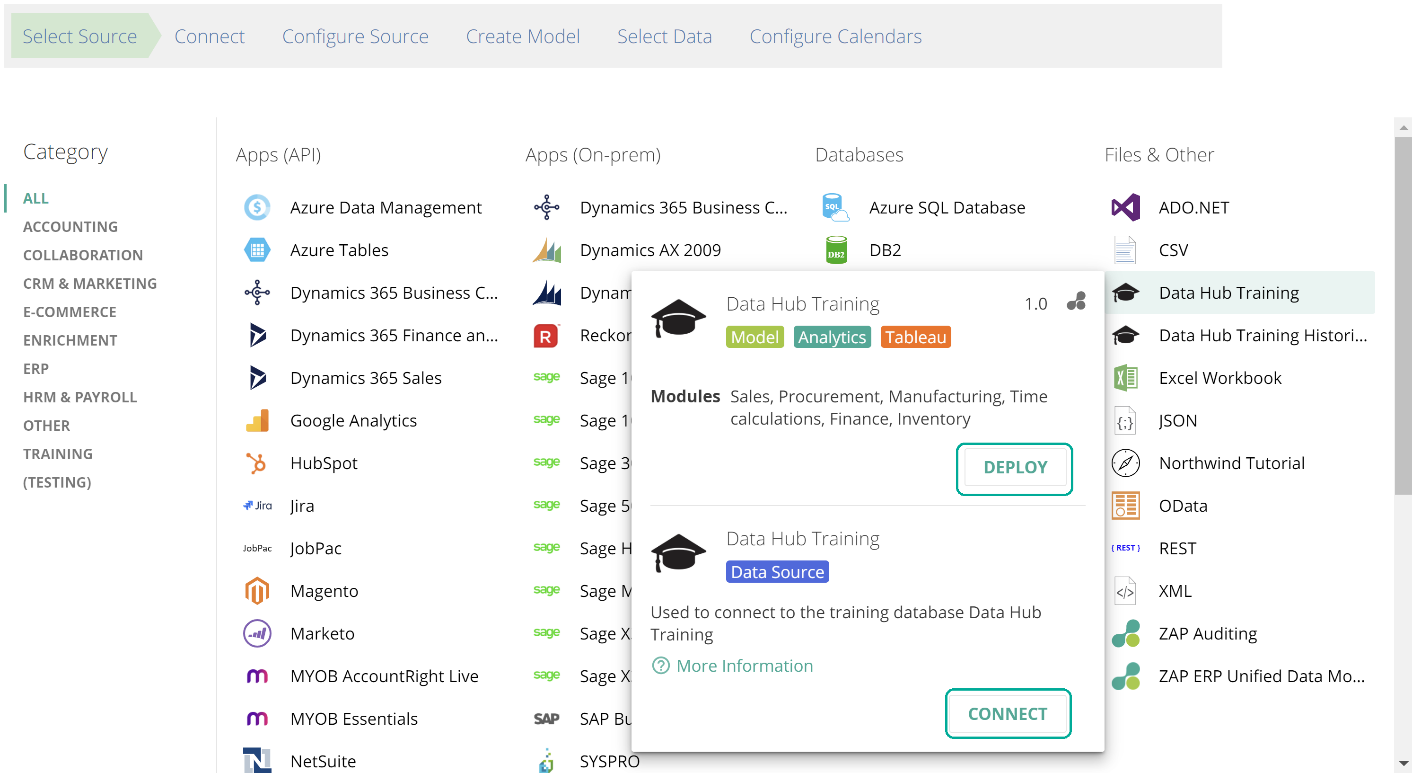
Select Source
You DEPLOY a Solution, and you CONNECT to a data source, as in the following image.
 |
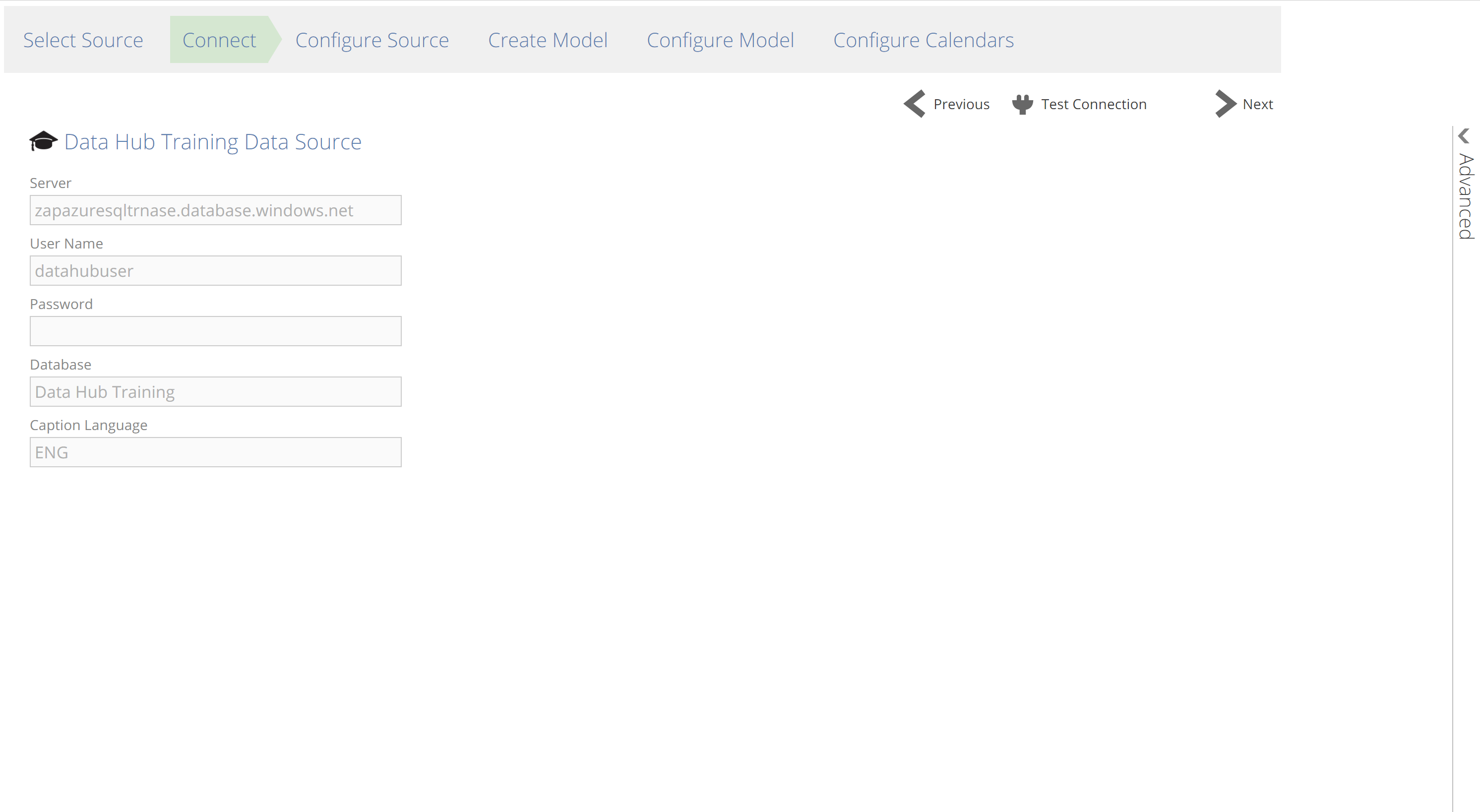
Connect
The Connect step is where you provide source connection details. The requirements for the Connect step range from no-requirements (as for the Data Hub Training data source and Solution) to quite comprehensive requirements (as for some financial sources).
 |
This step will require that you have in advance all prerequisites specific to your source:
Credentials – to the source with sufficient rights.
Deployed Data Gateway (optional) – for connecting to on-premise sources from cloud instances of Data Hub. The Data Gateway is a lightweight application that is downloaded from within Data Hub to simplify cloud connectivity. See the Connect to on-premise data article for steps to creating and installing a Data Gateway.
Additional source details – as required for some sources, and detailed in the relevant data source article (see here for the list of data source articles).
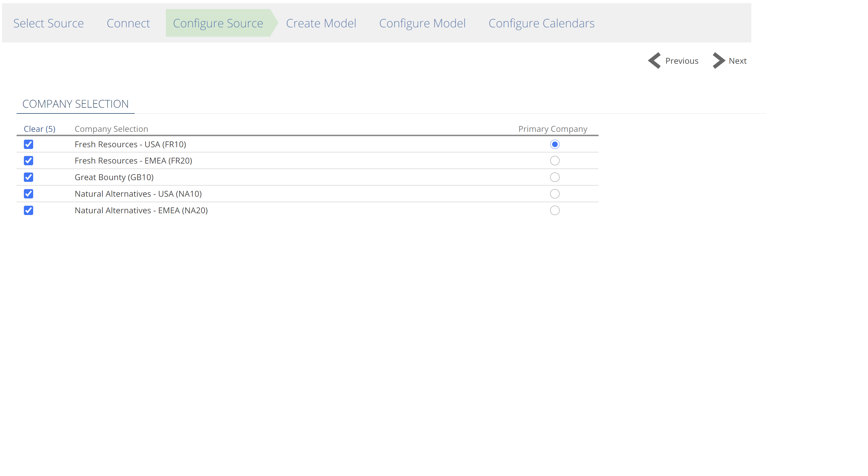
Configure Source (some sources only)
Once a connection has been established, the Configure Source step will show for some sources and provide source-specific configuration. A company selection is the most common source-specific configuration you will see.
 |
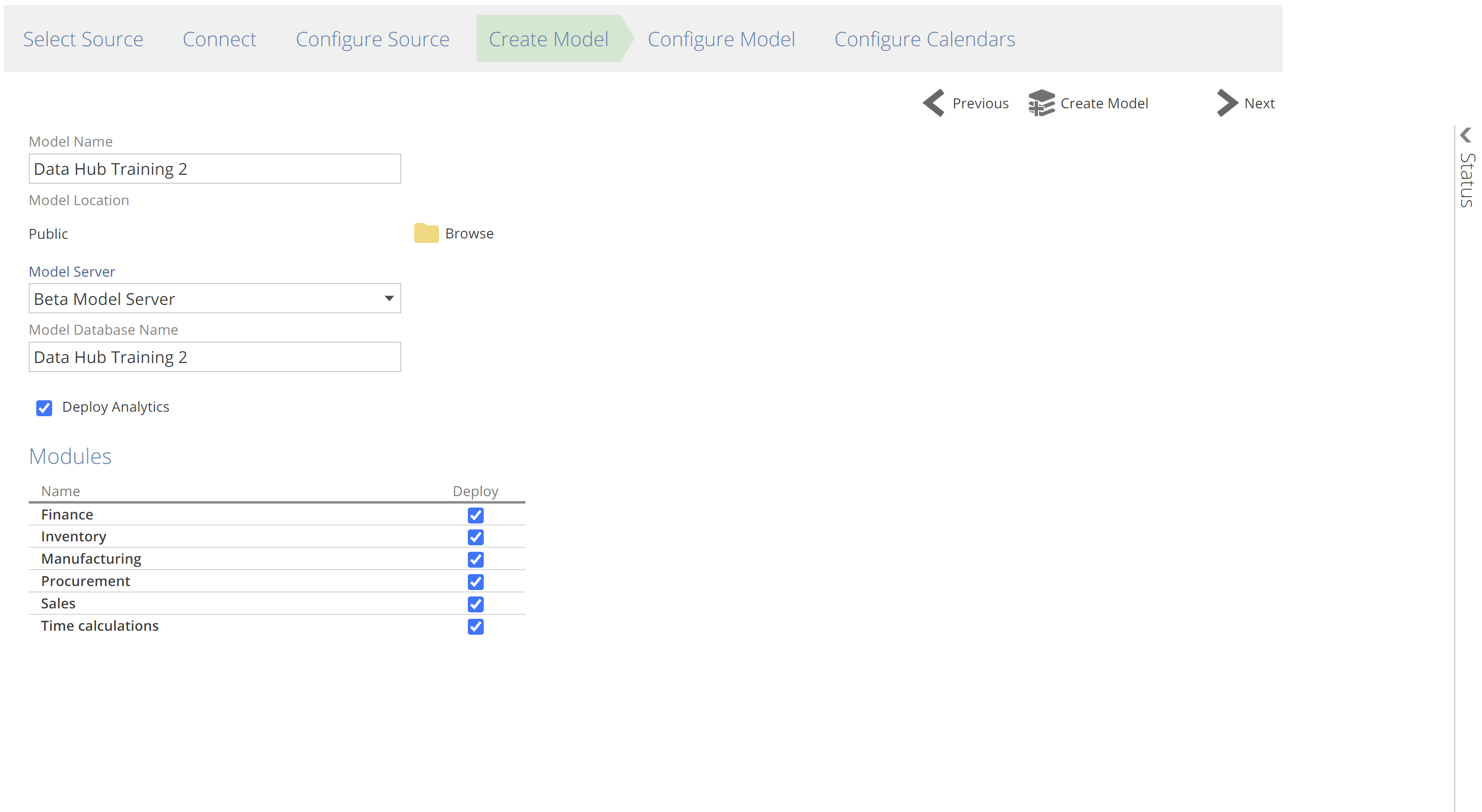
Create Model
Time to create the model. After this step, you will be able to see the Model resource and its related sub-resources in the Resource Explorer. There are options for the name and destination location of the new Model. For Solutions, two additional configurations are available:
Deploy Analytics – pre-built analytics are available for Power BI, Tableau, and Data Hub. If you wish to use Analytics with Data Hub, check this option to ensure the analytics are deployed.
Modules selection – as described previously, Modules are tagged groups of Pipelines you are choosing to include from the Solution in your new Model. You can also filter by Module in Pipeline lists on various tabs.
 |
Configure Model (some sources only)
At this point, the Model creation wizard may provide you with further source-specific options. Some sources categorize data across “dimensions”. The most common source dimensions are financial dimensions. The image below shows the financial dimensions sections for the Data Hub Training source. Do not confuse these source dimensions, with semantic layer dimensions (discussed in Complete Guide to the Semantic Layer (Coming Soon)).
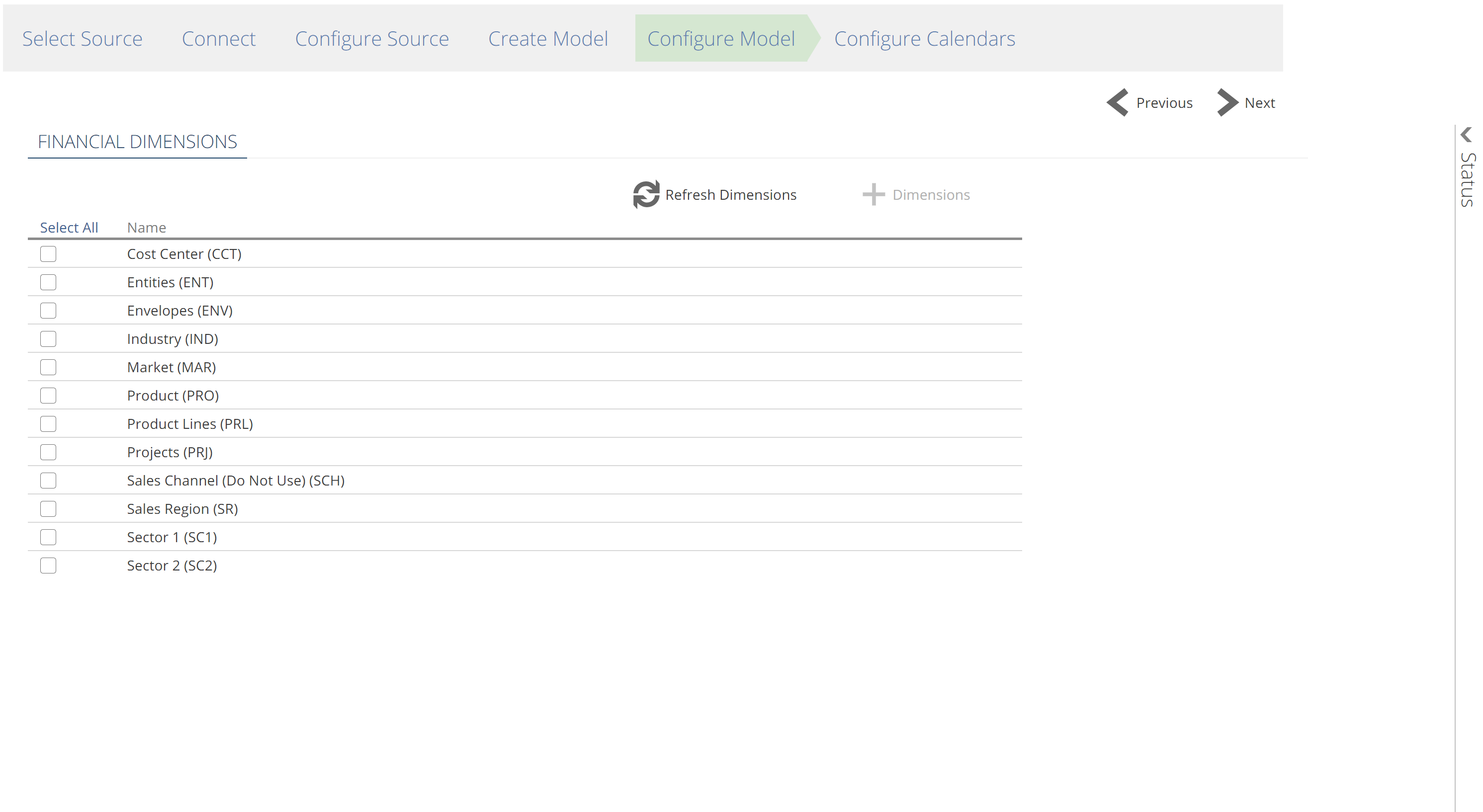 |
Select Data (data sources only)
If you created your Model from a data source (as opposed to a Solution), this is where you choose the initial set of Pipelines. You can, of course, add additional Pipelines after the model has been created. This step also allows you to preview your data by clicking the source tables (Data Hub considers each table, sheet, or API-endpoint to be a “table” of data).
You can add Pipelines in bulk by making your selection and then clicking Next, or you may choose to add your Pipelines in batches using the Add Pipelines button. To simplify adding in batches, you can filter the set of Pipelines and Select All (optionally for a filtered set of Pipelines). The batch technique ensures you don’t accidentally lose your investment in a complex selection.
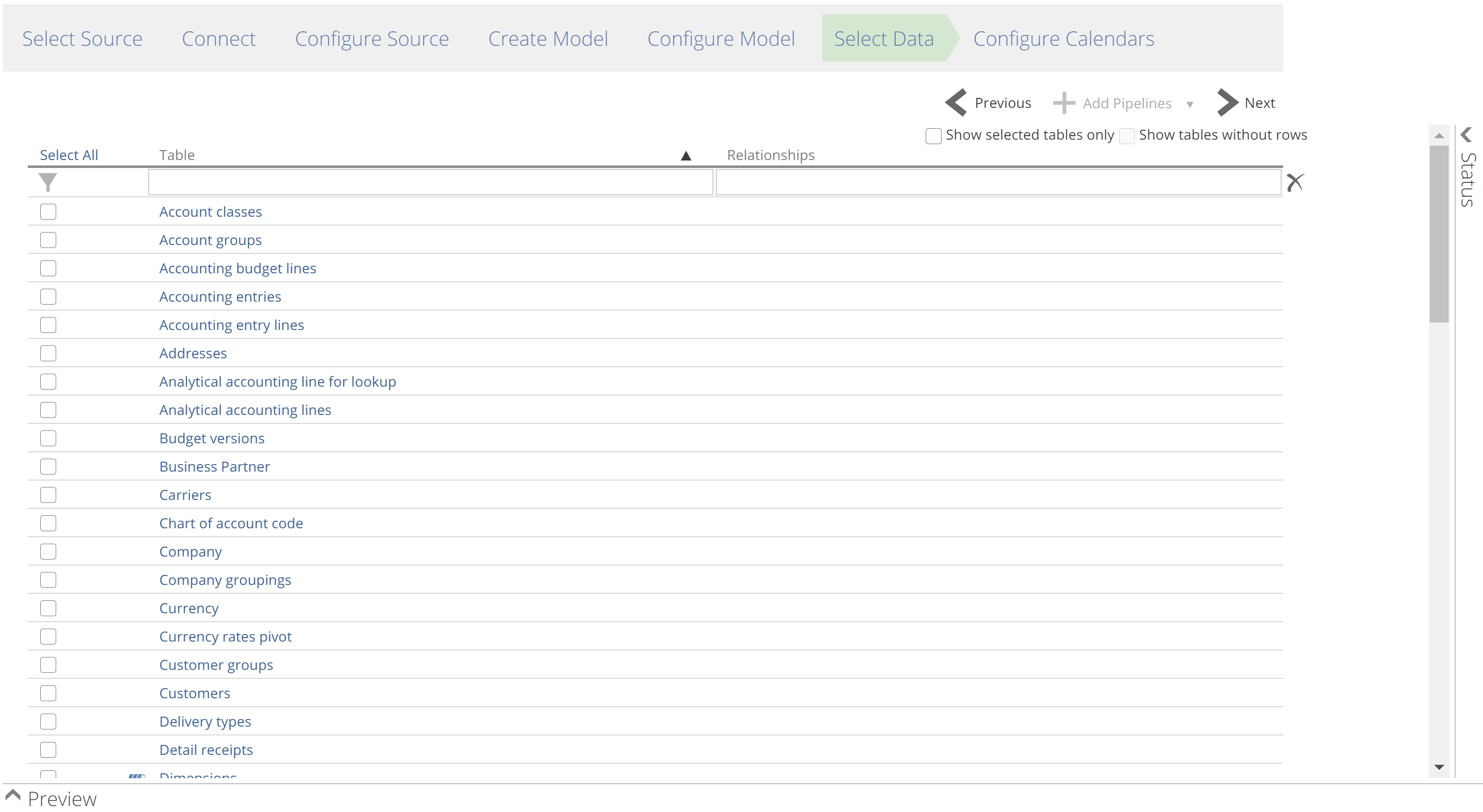 |
There is one other capability introduced on this step of the wizard, namely Table Merge. As the name implies, this allows you to combine (merge) the rows of similar tables by specifying two or more tables as the source of a single Pipeline. To use this feature, column names should be a close match.
Select the Pipelines to combine and click Add Pipeline as Union of Tables from the drop-down, as in the following image.
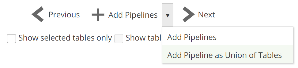 |
Configure Calendars
The final step of the Model creation wizard is to configure the system-generated Date Pipeline. There are three important configurations available on this screen (in addition to the Date format field):
The date range of the Date Pipeline – configured with the First day and Last day fields, this date range applies to all calendars.
The calendars available – four calendars are available by default (see image below) and each calendar supports customization from the Calendar design panel. Financial calendars offer a great deal of configuration, as detailed in Configure a Date Pipeline. Calendars can be added (by clicking + Calendar) and removed by right-clicking a calendar and clicking Delete.
The Global Date Filter – allows you to filter data from the source to the range provided. The Global Data Filter provides one of the simplest and most powerful solutions to optimizing a model. Importantly, only certain fact Pipelines are filtered (recall fact pipelines capture observations and events). Fact pipelines come preconfigured in Solutions. We will look at the specific requirements for the Global Data Filters to take effect later in this article.
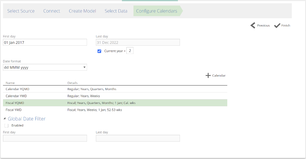 |
Once you have configured your calendars, click Finish. This will open the Model resource.
The Model resource tab
The Model resource is now shown on a resource tab. The Model resource is the starting point of navigation for most activities. Configuration is broken down into sections as in the following image.
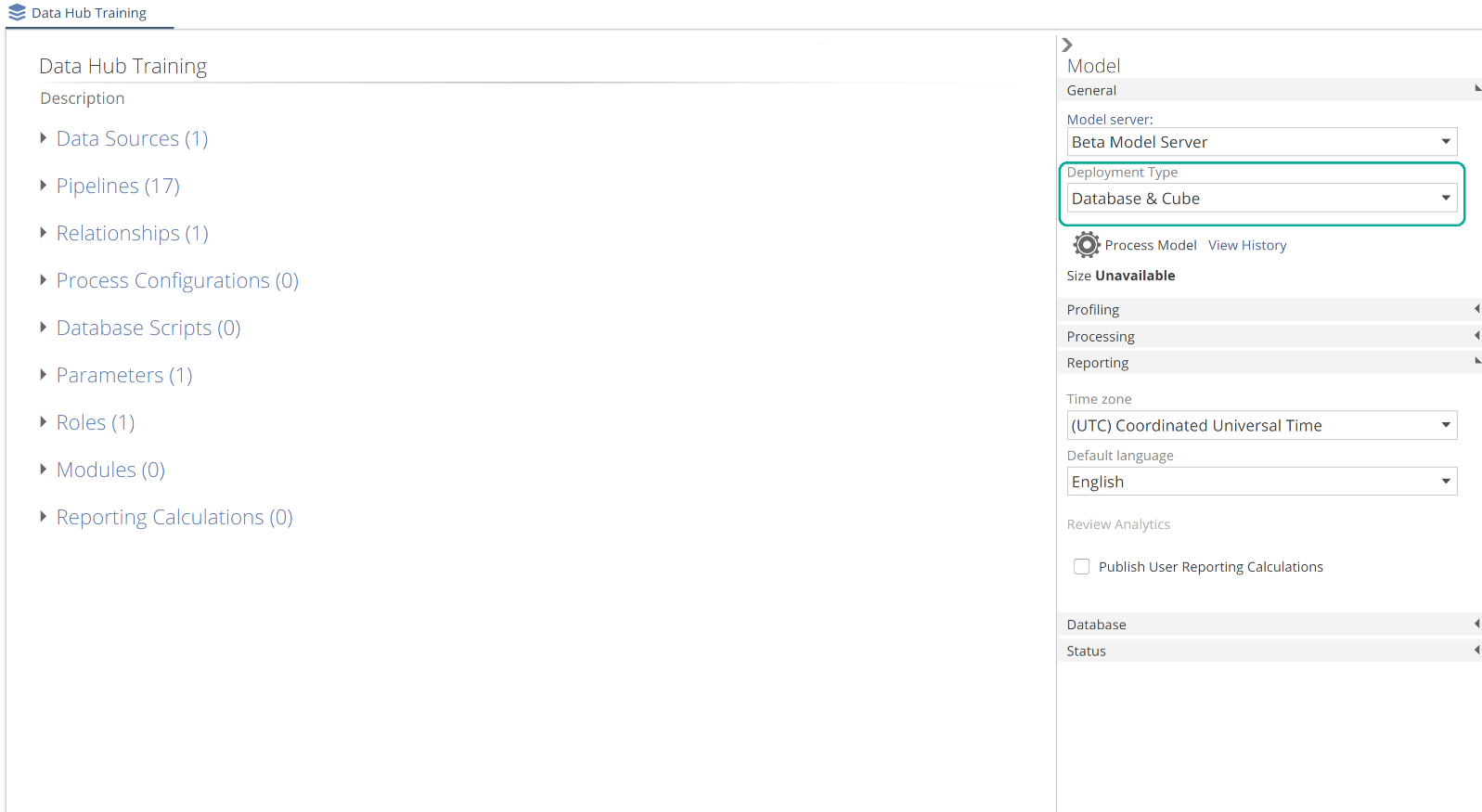 |
On the right-hand side of the Model resource tab is the Model design panel. At this point, you can choose whether you report against the warehouse or the semantic layer. If you are using Analytics with Data Hub or you plan to create custom analytics against the semantic layer, you should choose Database & Cube. Otherwise select Database. If you created your model from a Solution, you can click Process Model to build a complete warehouse (and optionally a cube).
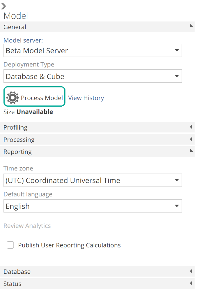 |
We will discuss the process model operation shortly and will also discuss most options from this panel in future sections. However, if you have been following through with this exercise in Data Hub, you can discover each option now by making use of the in-application tooltips. Simply over a label for in-application documentation in the form of tooltips. These tooltips also link to Data Hub’s online documentation. Following is a particularly rich tooltip for functionality we will look at shortly.
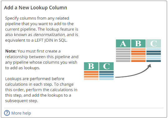 |
If you are using Analytics with Data Hub, you checked Deploy Analytics on the Create Model step, and you processed the model, you can begin working with your analytics. However, most likely you will want to customize some aspects of your Model, so read on.
A final point on the Model resource, as described previously, Data Sources and Pipelines are sub-resources of the Model resource. For this reason, it is also possible to navigate to these and other resources through the Resource Explorer. More information on this topic can be found in the Model organization using the resource explorer article. Viewing Model sub-resources through the Resource Explorer provides some additional capabilities, for example, the ability to copy and paste Pipelines within a model or between models. However, in general, it is best to navigate to Pipelines through the Model itself.
Data Hub architecture
Before we address configuring a Model, we need a quick foray into Data Hub architecture. Data Hub uses the Extract, Load, and Transform (ELT) process. That is, it:
Extracts the data from the source(s).
Loads it into staging tables.
Transforms it into a report-ready structure.
We previously touched on the concept of a schema with the introduction of the star schema approach to modeling. Let’s now introduce the concept fo a schema in full. Where a data model is a high-level plan for what a database should be, the schema is a description of what it is. That is, a schema is a realization of a data model. It should follow the plan and include the data. The warehouse that Data Hub generates consists of two schemas:
The staging schema that holds the staging tables for “staging” our data. Staging is used here in the same sense that “staging” for a play or film involves selecting, designing, and modifying a performance space. So, this is where we stage our data for the final performance.
And the warehouse schema is that final performance. It holds the warehouse tables for end-user reporting or for the semantic layer to query those tables (so that the semantic layer may serve as the end-user report database). Be careful not the confuse the warehouse schema with the warehouse itself (which holds both the warehouse schema and the staging schema).
We’ve used “table” loosely in the above because many, if not most, of the tables in each schema, will be virtual tables or views. A view is a virtual table in the sense that you can query it as you would a standard table. However behind the scenes, instead of being defined by its column names and column data types, a view is defined by a saved query in the database. When data is requested of the view, it evaluates this saved query. The saved query of a view can in-turn refer to another view, and that view may refer to yet another, and so on. In this way, layers of views can transform staging-table data into warehouse-table data.
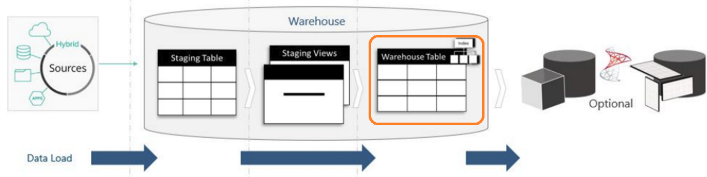
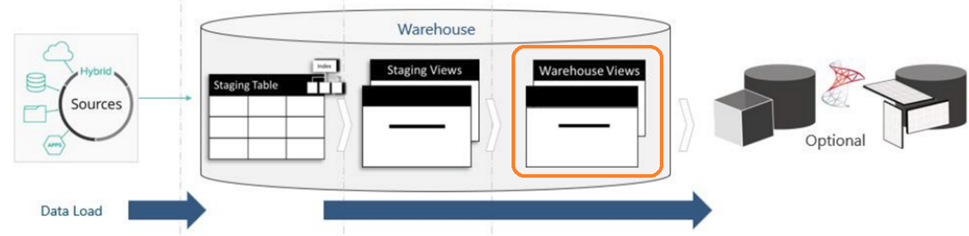
Let’s expand on this brief introduction with the assistance of the following architecture diagram. We will discuss each concept in turn.
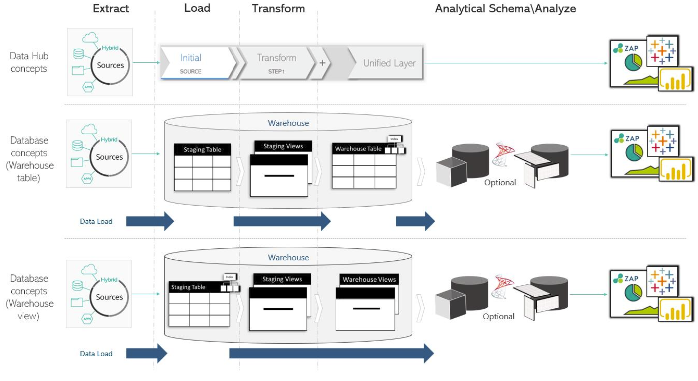 |
Extract
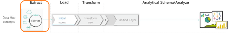 |
The Extract step entails retrieving raw data from the source system. Consider it the “copy” from the copy-paste operations you would use when editing documents. To extract the data, Data Hub connects to a multitude of sources (see here) using a variety of techniques, including:
Web services – a large selection of web services are supported, in addition to generic capabilities to support those services not already available.
Databases – including support for all major on-premise and cloud database vendors.
Files – for CSV, Excel, JSON and XML sources.
Hybrid – for some sources, Data Hub makes use of a database connection in parallel with web service connections. This hybrid approach provides an even richer source of data for reporting.
If Data Hub is hosted in the cloud, then the database, file, and hybrid connections will make use of the Data Gateway. Recall, the Data Gateway is a lightweight application that is downloaded from within Data Hub to simplify cloud connectivity.
While most data transformation is performed in the staging schema (as the Extract, Load, Transform process suggests), it is possible (and occasionally) optimal to ask the source itself to perform some of this transformation at extract time. The main requirement for such out-of-step transformations is to shape the data to the extent that it supports filtering that might not otherwise be possible. This filtering then allows Data Hub to extract the optimal volume of data. We will see how this is done in a future section.
Load
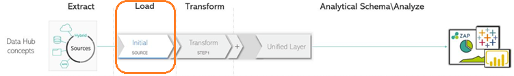 |
What the Extract step is to “copy”, the Load step is to “paste” (from our document editing analogy). Data is “pasted” directly into the staging tables of the staging schema. Data Hub breaks the data Pipeline down into Steps. From the image, we see three example steps (Initial, Transform, and Unified Layer). We will talk to each of these. The Initial Step is where the designer chooses which columns to load from the source.
Transform
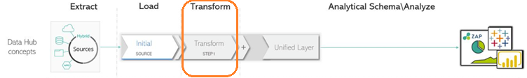 |
The transform Steps are those after the Initial Step, excluding the Unified Layer (which we will talk to shortly). In this diagram, we have unimaginatively named the sole transform step “Transform”. The transform steps are where the designer stages the data (recall our film analogy). And recall the transformation itself is performed by views (virtual tables) in our staging schema. Each data Pipeline Step may generate one or more views, as we will see later. The staging and warehouse schemas are described in more detail in the following.
The staging schema has two sets of objects:
The staging tables – hold copies of source data for each data Pipeline.
The staging views – capture the transformation logic for each Pipeline.
The warehouse schema also holds two sets of objects. However, each Pipeline has either:
A warehouse table – that holds transformed data as a result of querying the final staging view.
A warehouse view – that is a direct query of the final staging view. A warehouse view provides an on-demand transform option.
We “migrate” data from the staging tables to the (optional) warehouse tables. This terminology avoids confusion with “loading” data into the staging tables. The Model designer configures whether each data Pipeline results in a table or view. More on this shortly. The optional Unified Layer Step standardized Pipeline properties such as column names and column data types.
There is also an additional history schema, that holds tables of historical data for each data Pipeline with the special History step. The history schema serves a similar purpose to the staging schema, but for historical data. We will talk about the History step in a future section.
Processing & publishing
Having described the objects themselves, we can now cover the data flow. Data Hub refers to refreshing the data as “processing”. There are three types of processing:
Source processing – data is loaded from the source systems to the staging tables.
Warehouse processing – data is migrated from the final staging view to the warehouse table (but only for Pipelines the designer has configured to result in a table).
Semantic layer processing – data is migrated from the warehouse tables and views to the semantic layer. Data is only migrated for data Pipelines marked for inclusion in the semantic layer.
In the following excerpt from our diagram, note that the final warehouse object is a warehouse table.
 |
This image shows the data flowing from the source to a staging table, from the staging table to a warehouse table (through the transform views), and from the warehouse table to the (optional) semantic layer.
The following excerpt shows the alternate data flow, where the final warehouse object is a warehouse view.
 |
This image now shows the data flowing from the source to a staging table, and then from the staging table to the semantic layer (through the transform views on demand). Sensibly there are performance and storage considerations to choosing between warehouse tables and warehouse views.
All processing types can and should be performed incrementally after the initial full load. Incrementally means we only load or migrate the new or updated rows. These topics will be covered in future sections, and a complete performance tuning guide is also available in the online documentation.
Benefits to the Data Hub approach
Before moving on to how a Model is configured in the Data Hub application, let’s quickly review the benefits of the Data Hub approach:
Extract & Load
Transformations do not place a load on source systems.
Transform
All transforms are performed with a common modeling approach, levering the power of Azure SQL or Microsoft SQL Server.
Changing a data model does not require re-migration of all data.
While Extract, Load, Transform does entail some double storage, Data Hub supports column compression technologies. In some cases, this compression can also result in improved performance.
And that’s it! It is recommended that you take the time to digest these concepts fully. With this knowledge properly bedded in, you will be in an excellent position to model data in Data Hub. From here, we will return to our newly created Model, and look at how to customize it to your requirements.
Now, data extraction (the first step from Extract, Load, Transform) can be very technical. However, Data Hub automates all data extraction based on the Model’s configuration. And having walked through the Model creation wizard most of this configuration is now in place. We will return to data extraction late in this article in the Data Sources section. However, we can now focus on loading our data.
Data Loading
Pipelines
Recall that most modeling is performed against the Pipeline resources of the Model. And so, it is with Pipelines that we start.
From the Model resource tab, you navigate to Pipelines from the Pipeline list. This list provides various filtering options for use with large models. You can see an “account” filter applied in the following image.
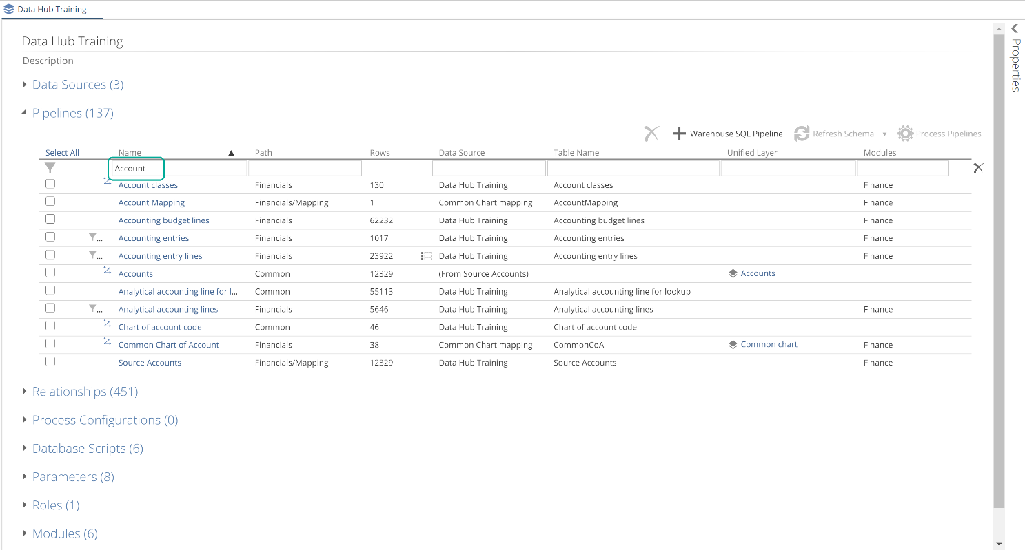 |
As you can see, the Pipeline list is also where you delete Pipelines. We will cover the other sections from this image throughout this article. On opening a Pipeline, the COLUMNS tab is selected, and the last step is active. This last step is often the Unified Layer Step, as in the following image.
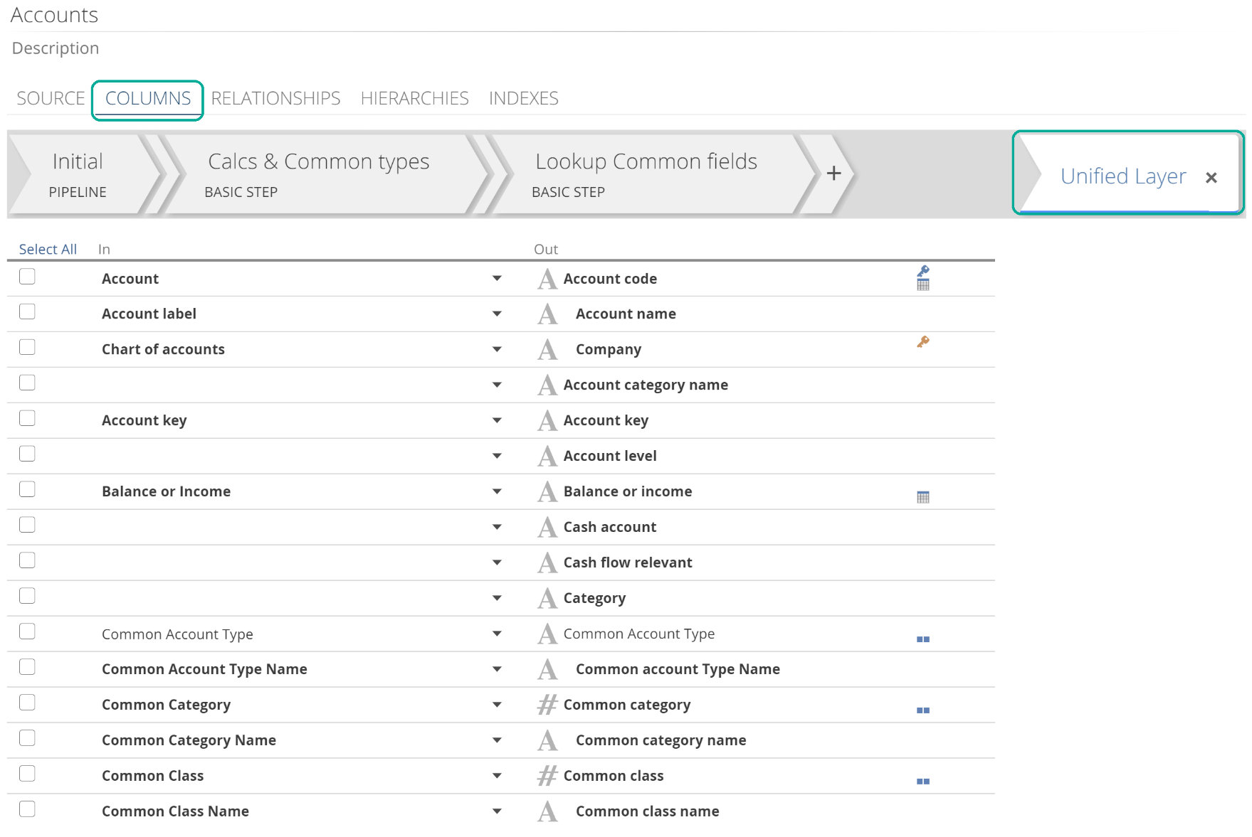 |
The columns list shows for this step and reflects the transformed result of the entire Pipeline.
At this time we’re interested in loading the data, so we turn to the SOURCE tab (to the left of the COLUMNS tab). The SOURCE tab defines the source and allows you to control the rows to load. The Initial step (which we will talk about shortly) allows you to define the columns to migrate.
SOURCE tab
We selected our initial set of Pipelines using the wizard. Pipelines were either selected individually or in groups (by Module). Either way, the model creation wizard preconfigured each Pipeline’s Data Source and Tables, as in the following image.
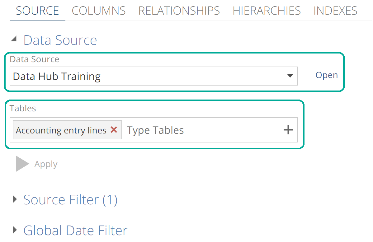 |
If you made use of Add Pipeline as a Union of Tables for a Pipeline, you will see more than one table in the Tables field.
While the SOURCE tab allows you to change the Data Source and Tables for a Pipeline after Model creation, the most common configuration performed on this tab is source filtering using either the Source Filter or Global Date Filter sections. The benefit to source filtering (as opposed to Step filtering which we will see shortly) is that it reduces the volume of data to be loaded from the source. Source filtering is available for most, but not all sources.
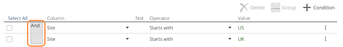
To define a source filter, expand the Source Filters section and click + Condition to add to the conditions list. You can group conditions (and create groups of groups). Grouping is performed by selecting the conditions and clicking the Group button. You can then toggle the Boolean operator for the group by clicking on it as in the following image.
 |
Negation is similarly a matter of toggling the Not button (it doesn’t show until you hover in the column). Newly added conditions compare columns to values, but you can change a condition to a column-to-column or column-to-parameter comparison by clicking on the vertical ellipsis, as in the following. We will discuss parameters in a later section.
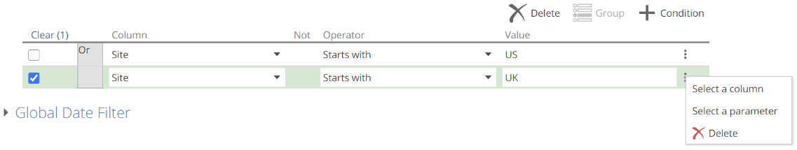 |
The source Preview section provides a filtered preview of source data to support the building of filters. We will address the Preview section in detail when we discuss Steps.
The other means of source filtering is to use the Global Date Filter. Recall that the Global Date Filter was configured at the model level on the Configure Calendars step of the Model creation wizard. You must also specify the individual Pipelines to which the Global Date Filter will apply. This is only a matter of checking Enable and optionally specifying a Date column on those pipelines. As always, if you need information on how particular functionality works, hover over the relevant label, as in the following.
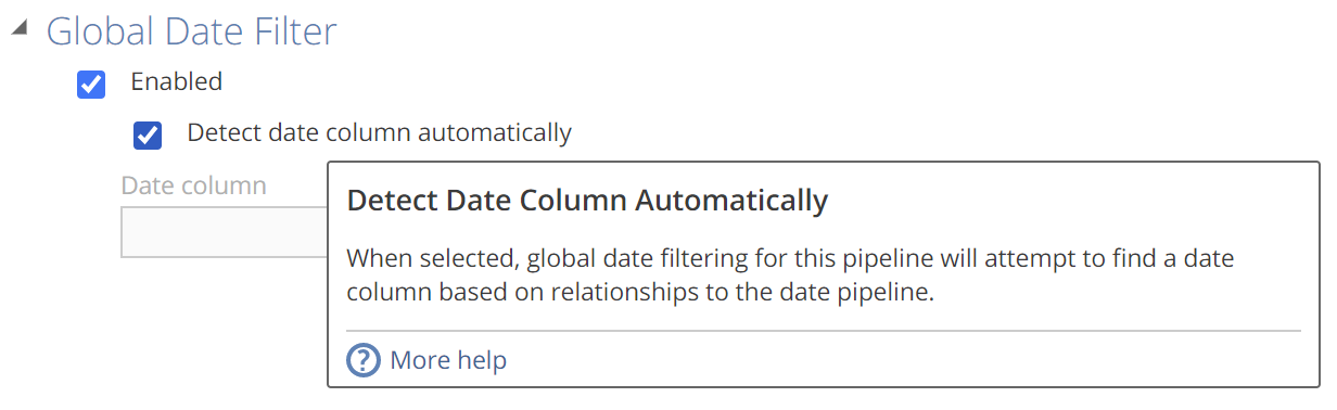 |
From the tooltip, we can see that if you check Detect Date Column Automatically, then then you will need reporting relationships in place, which is a topic we will address later.
Before moving on, it is worth noting that the SOURCE tab can differ across source types. For example, CSV-sourced Pipelines don’t provide filtering options. They do, however, provide CSV-specific options. Such options include overriding the delimiter character.
The Initial step
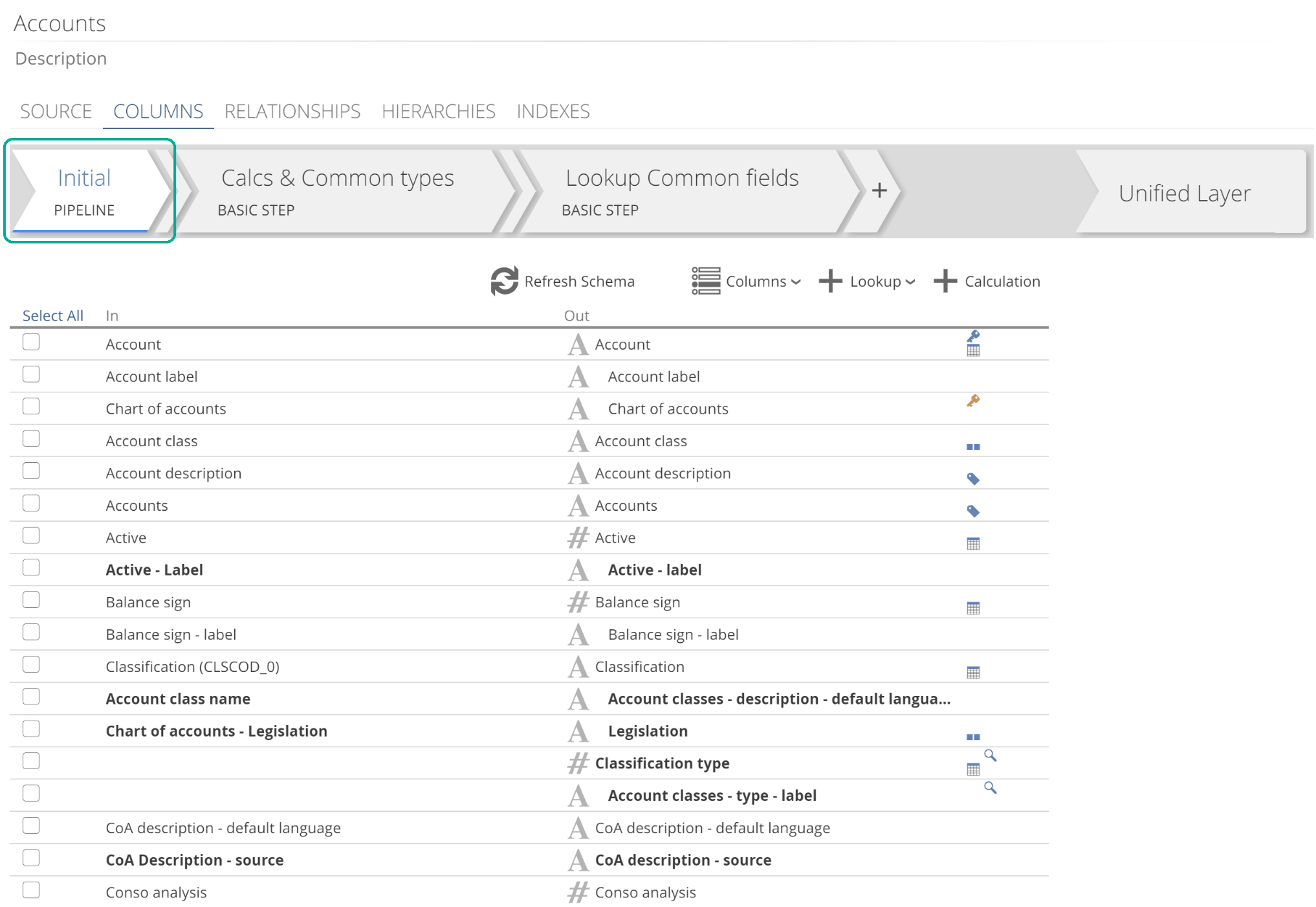
Having configured the rows for migration using source filters, the Initial Step allows us to configure the columns to load. For the Initial Step, we return to the COLUMNS tab, as in the following image.
 |
The columns list shows an initial selection of columns based on automatic data profiling. You modify the selected columns by clicking Columns, as in the following:
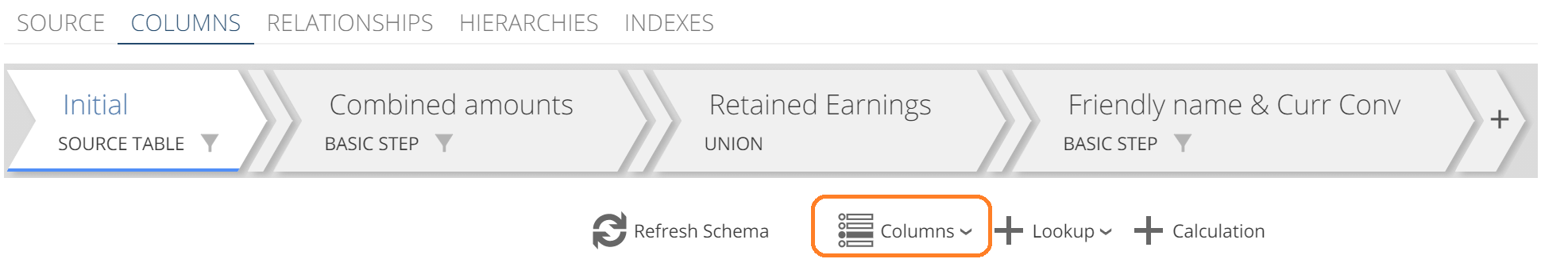 |
We will discuss the Refresh Schema button when we cover Data Sources as this option is available both on the individual Pipelines and the Data Source itself. Now, having clicked Columns, the Source Columns checklist shows. Make your selections and click Apply.
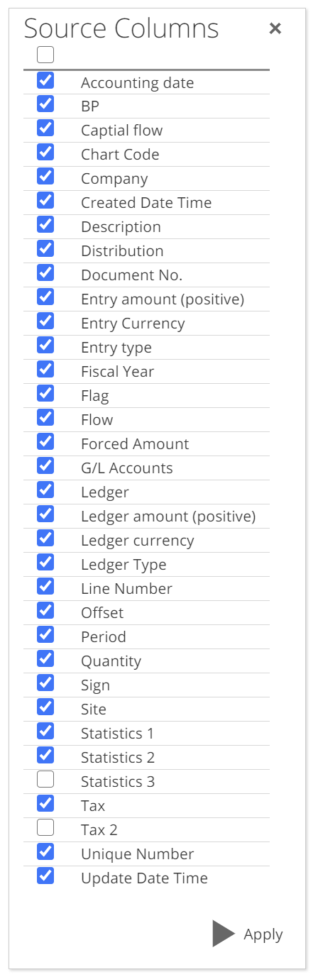 |
The Initial Step serves one more important purpose. It defines the keys of the staging table of the Pipeline. The key of a database table grants you access to a specific row of that table (and not the table itself). It does this by specifying columns that will uniquely identify a row. So the key of a table is one or more columns that will uniquely identify any row in that table. For example, the key of a Customer table could be the Customer Id column, or it could be the Customer IdandCompany columns. This latter combination of columns would be required if the Customer Id column alone would not suffice to uniquely identify a row. As with default column selections, keys are often preconfigured by Data Hub.
The following shows the keys for the Accounting Entry Lines Pipeline from the Data Hub Training Solution. We will make use of this Pipeline for a few of the examples to come.
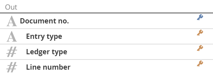 |
Keys on the staging table are essential for incremental source processing because to update a row, Data Hub must be able to uniquely identify it. Recall incremental processing means we only load the new or updated rows.
Incremental source processing
With the Pipeline keys in place, let’s take a quick look at how to configure incremental source processing. We will discuss incremental warehouse processing separately in the Optimize section of this article. Configuring incremental source processing is relatively simple, but it is also one of the most effective model optimization techniques available. For these reasons, it is worth configuring incremental source processing as soon as you start working with your model. That is unless you created your model from a Solution, in which case these settings come preconfigured.
Incremental source settings are configured on a Data Source for all Pipelines sourced from it. And each Pipeline has the option to override these settings. Configuration at both levels is very similar. We look at pipeline incremental configuration now, and we will look at Data Sources incremental configuration shortly.
All Pipeline settings are configured on the Pipeline design panel, shown on the right-hand side of the Pipeline resource tab. The Pipeline design panel is available from any tab (SOURCE, COLUMNS, etc.), provided no list items are selected. If a list item is selected (for example a column on the columns list), then the design panel will show settings appropriate to that selection. The Pipeline design panel is shown below with only the Incremental Process (Source) section expanded.
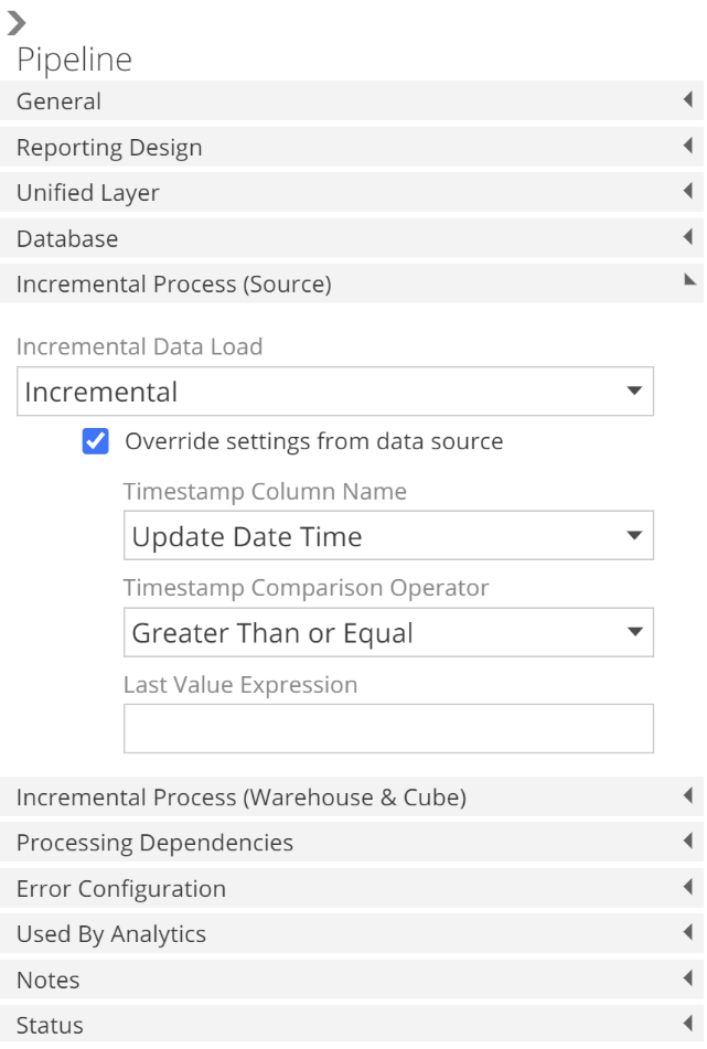 |
Turning to configuration, if you are overriding the Data Source default, you must first check Override settings from the data source. The basic operation of incremental source processing is to extract from the source only those rows that have been added or updated, based on a source timestamp column. And the most common reason to override the Data Source default is that the source table for the Pipeline in question does not have the timestamp column specified on the Data Source.
Having checked Override settings from data source, you may now override the Timestamp Column Name for this Pipeline. From the image, you will note there are further configuration options available in this section. These options provide additional flexibility, but they are beyond the scope of this article.
It is important to understand that a full data load will still be performed on any of the following conditions:
A filter is changed on the SOURCE tab. For this reason, it can be a significant time-saver to get the source filter right the first time.
Additional columns are selected on the Initial step.
The Global Date Filter settings are modified on the Pipeline or in the master configuration on the Date Pipeline.
The Tables specified on the SOURCE tab are changed.
Occasionally specific source tables for a source system do not have the required fields to support incremental source. In this case, the Incremental Data Load drop-down provides the following two options:
Full Refresh – Always re-load all rows from the source.
Load Once – Perform a full refresh on the first load. Subsequent loads will be skipped.
Finally, some source tables are, by their nature, subject to data deletions. There is no issue if a row is simply marked as deleted and the timestamp is updated at the time. However, Data Hub cannot identify rows that have been physically deleted. The most common scenario for this is where a table has a companion historical table. Periodically data may be deleted from the current table and inserted into the historical table. By using the Table Merge feature we saw previously on the model creation wizard, it is possible to incrementally load the combined source data (assuming a timestamp column exists in both tables).
This is an excellent point to introduce the Data Source resource tab.
The Data Source resource
Assuming you have a common timestamp column across most source tables, then the Data Source resource is where you can set this column as the default for incremental source processing. Open the relevant Data Source from the DATA SOURCES section of the Model tab and refer to the design panel on the right. The Timestamp Column Name field is available at the top, as in the following image.
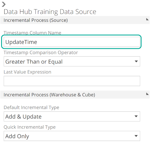 |
The Timestamp Comparison Operation and Last Value Epxressoin fields are also available at the Data Source level for additional flexibility should you need them (and as usual, hover for rich in-application documentation). We will talk to warehouse and cube incremental processing later in this article.
Looking around on the Data Source resource tab, note the Connection Details section is collapsed by default and includes the details entered on the Model creation wizard. Below that, the TABLES tab shows by default. There are additional tabs that will be discussed in time, including some that mirror the configuration available on the Model creation wizard. For example, the COMPANY SELECTION and FINANCIAL DIMENSIONS tabs, as in the following image.
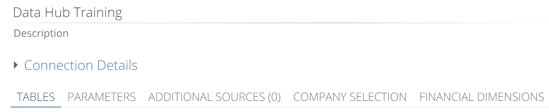 |
Adding pipelines
Staying on the Data Source TABLES tab, you will commonly want to add additional Pipelines for a given Data Source, after completing the Model creation wizard. This is done from the tables list, as in the following image.
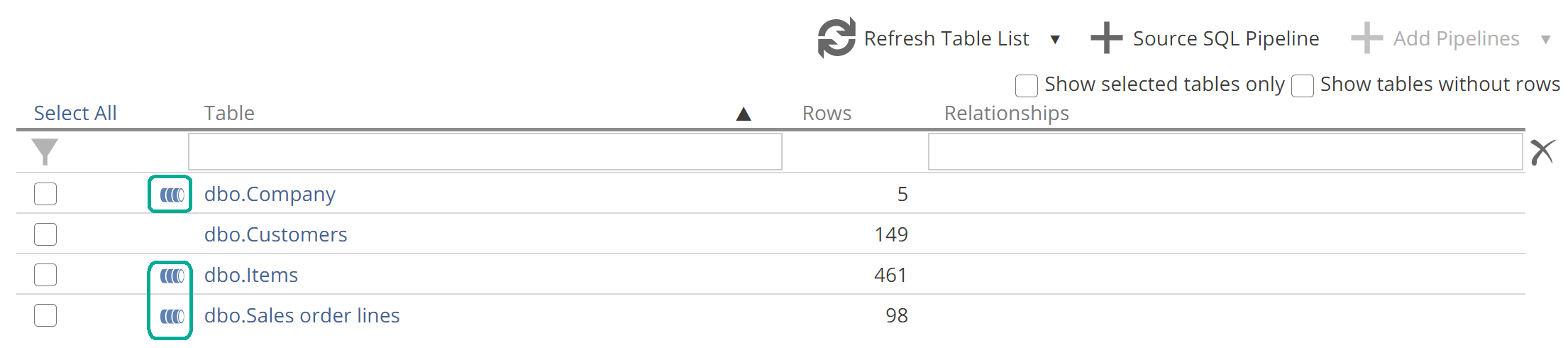 |
Source tables for which a Pipeline already exists will show a Pipeline icon as in the image. Select the Pipeline(s) you want to add and click + Add Pipelines. At this point, Data Hub will profile the data and automatically create relationships. The Add Pipeline as Union of Tables option is available from above the tables list, as on the model creation wizard’s Select Data step. You may note the option to create Source SQL Pipelines. We will touch on this option in a future section. There are also a few filtering options available for the tables list, and the in-application documentation should provide all the guidance you need for these.
Refreshing the source schema
We do need to discuss the Refresh Table List option.
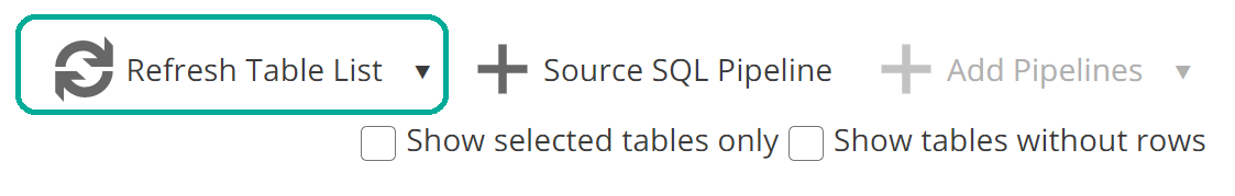 |
Each Data Source holds a snapshot of the tables list for its source. And each Pipeline holds captures a snapshot of the column names and columns data types for its source table(s). The Refresh Table List and Refresh Source Schema options allow you to update these two snapshots respectively. The details are as follows:
Refresh Table List – Refreshes the snapshot of tables held by the Data Source and shown in the tables list.
Refresh Source Schema – Refreshes the snapshot of tables held by the Data Source, in addition to refreshing the snapshot of column names and data types held by each Pipeline. If required columns have been removed or renamed, then the affected pipelines will now show validation errors.
You also have the option to refresh the source schema on individual Pipelines from each Pipeline’s SOURCE tab. However, the benefit of performing this in-bulk on the Data Source resource should be obvious. There are two main triggers for using Refresh Source Schema:
Known source changes – You are aware that significant changes have been made to the structure of the source system.
Model-category process errors – On occasion, a Model process will fail because of structural changes on the source. This will result in a Model-category error (which we will discuss) that provides instructions to refresh the source schema.
The usual trigger for using Refresh Table List is that you are aware a table has recently been added to a source and you require a refresh of the tables list. In this case, you want to make use of the faster Refresh Table List option because you are confident existing column names and column data types have not changed.
Data Modeling
At this point, we have selected the rows and columns to be loaded into our staging area. We have also configured the model to only load the incremental changes from the source. We are now ready to start transforming our data, or as we introduced previously, modeling our data. It’s a must nicer word, after all.
Most modeling involves looking up values from one table to another, calculating new columns, and filtering rows. These task types are performed across the Initial and subsequent Steps.
Task views
Recall from that Data Hub uses a series of views to transform the data. Each Pipeline Step generates a task view for each task type. For example, a Pipeline with two Steps would have two sets of task views. And if each of those Steps used all three of the task types described, there would be six views.
The order of the task views is as follows:
Lookups
Calculations
Filters
The importance of this order is that a task type must be after or downstream of another task type to make use of its value. Let’s look at a few examples:
A calculation on one Step can reference a lookup from the same Step. The calculation task view is after the lookup task view and is therefore downstream.
A calculation on one step, cannot reference another calculation from the same Step. The latter calculation would be defined on the same task view and is therefore not downstream. We will see how to address this shortly.
A filter on one step can reference a calculation from the same Step. The filter task view is after the calculation task view and is therefore downstream.
We will walk through these examples and more in the following sections. However, don’t worry about remembering the rules. Data Hub will always guide you on what is possible. The point here is to understand the concept of task views so that you can make the correct decision when required.
Lookups
We have alluded to lookups, but let’s now provide a definition. A lookup is a new column on a Step, where each row’s value for that column is looked up from a row and column of another pipeline. For example, a Customer Pipeline may include an Address lookup on the Initial step, that retrieves its relevant values from the Address column of a Customer Address Pipeline. A lookup requires a predefined relationship between the host Pipeline (Customer) and the lookup Pipeline (Customer Address).
Let’s quickly look at configuring relationships in Data Hub before we create our lookup. The following image shows the RELATIONSHIPS tab with two configured relationships for the Accounting Entries Lines Pipeline from the Data Hub Training solution.
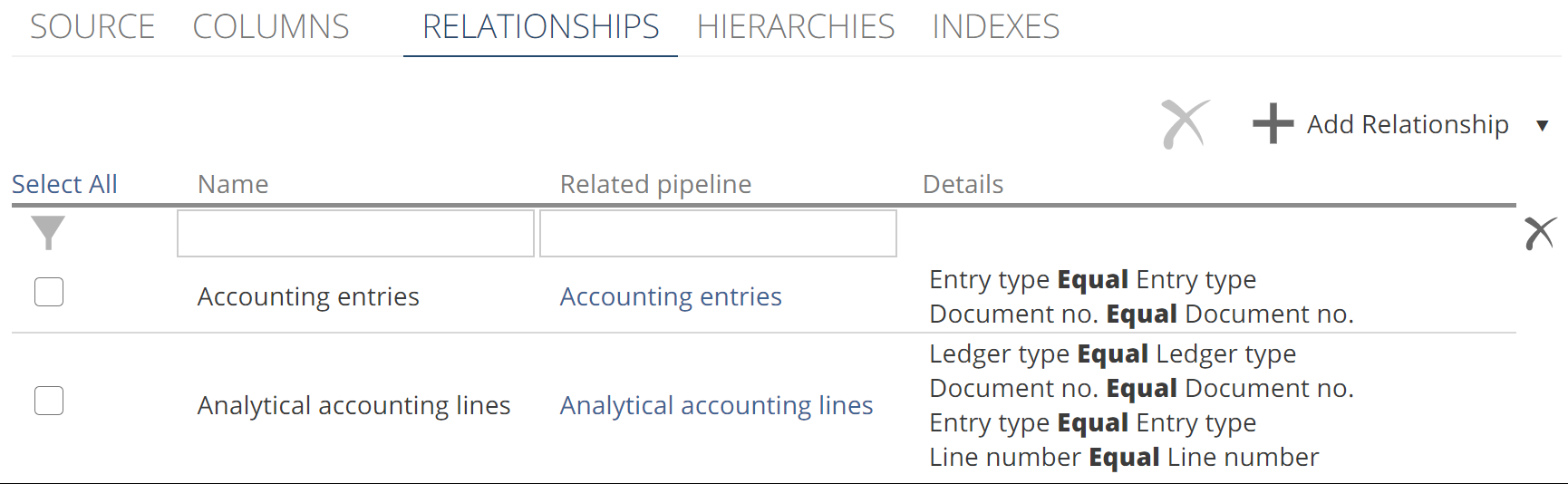 |
You add a relationship by clicking + Add Relationship, but in this case, let’s work with the relationships already defined by the Solution. As you may be comfortable with by now, you select a relationship from the list to show the relationships design panel. The following image shows the relationship design panel for the first relationship from the list.
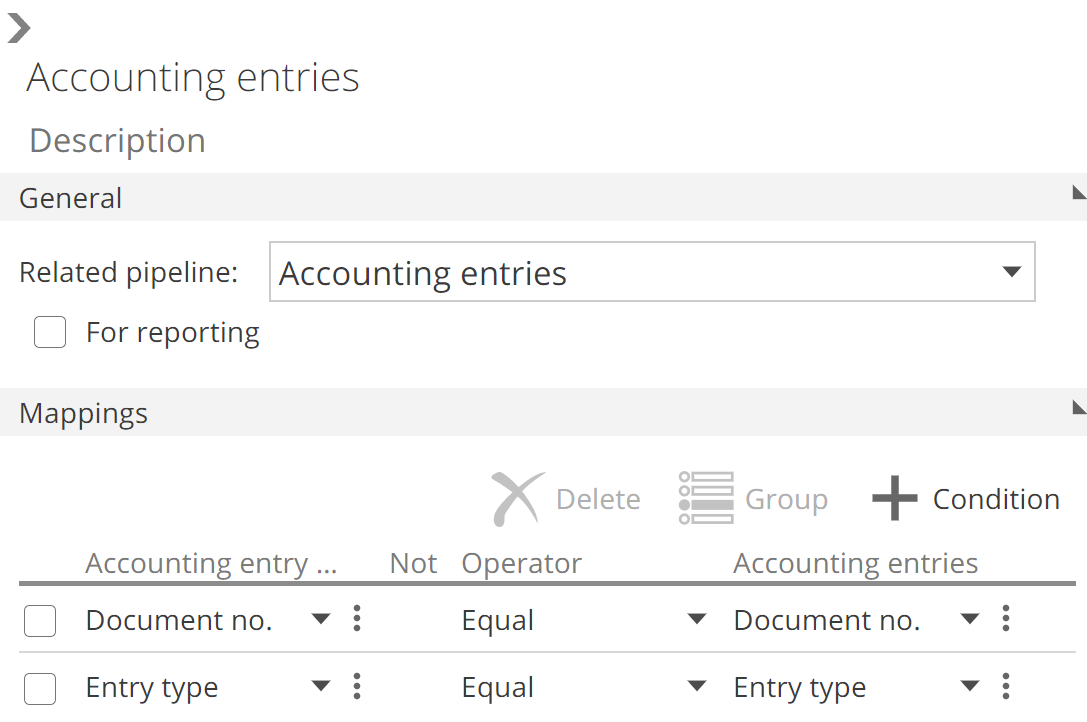 |
The most important settings from the relationships design panel are the Related Pipeline drop-down and the Mappings section. Mappings are configured using the same interface as filters. Operator, negations, and groups are all defined the same, and the vertical ellipsis changes the entry between column, value, and parameter. You can also change the relationship name and description at the top of the design panel. We will discuss the For reporting check-box in a later section of this article.
Having ensured our relationship is in place, let’s now create a lookup. Return to the COLUMNS tab and importantly for this example, select the Initial Step. Click the +Lookup button and browse the list of Pipelines. Expand the required Pipeline, select the desired column(s) and click Add. The following image shows a single lookup (Category) created on the Initial step.
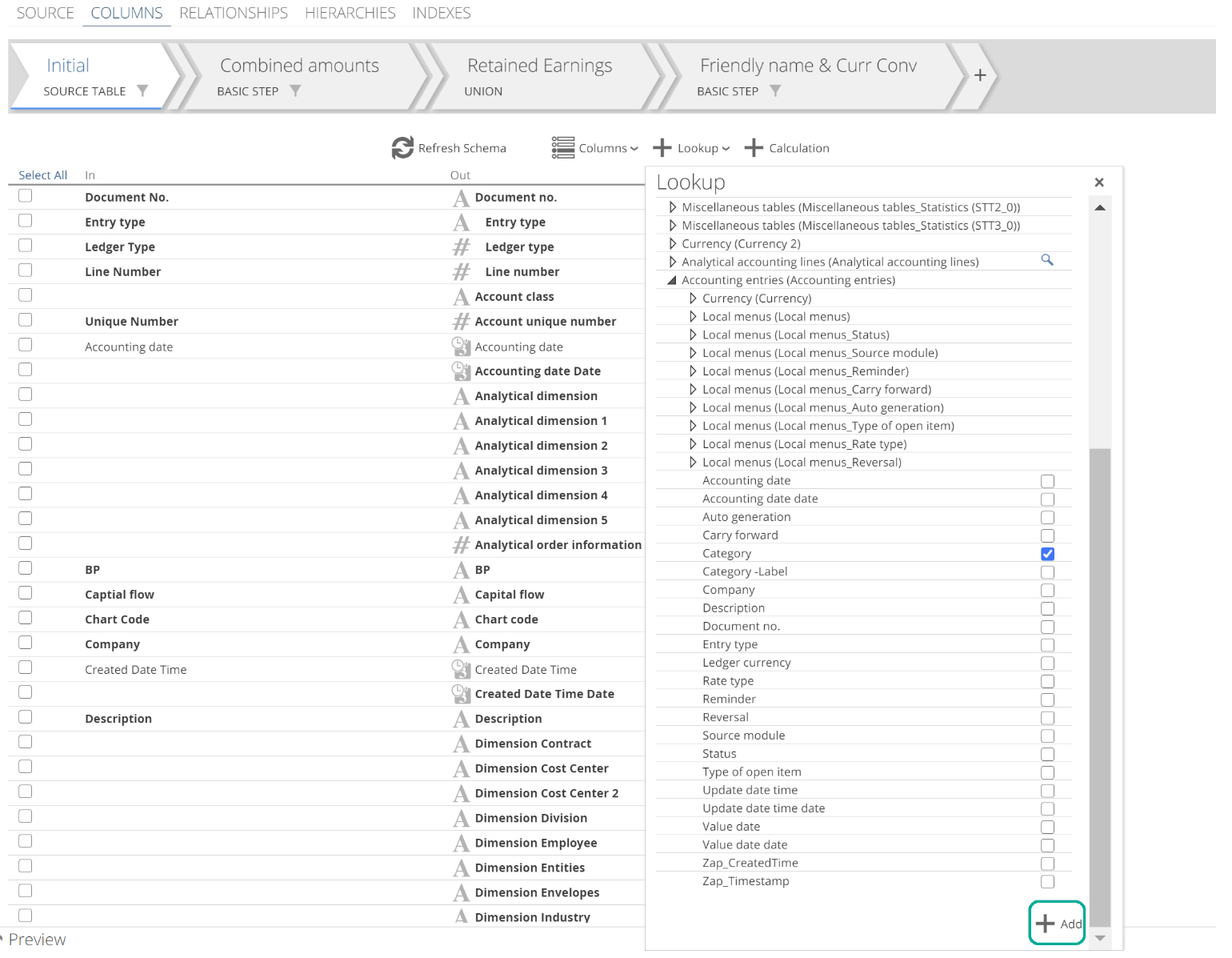 |
The name of the relationship used to relate each Pipeline is provided in brackets because it is possible to relate to a single Pipeline in multiple ways.
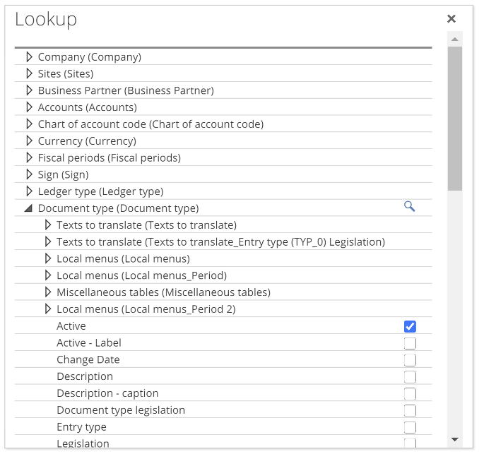
Now open click + Lookup again from the Initial Step and this time note that some Pipelines show as dimmed. If you hover over these, Data Hub will tell you that you must create lookups from this Pipeline on a subsequent step. This is the case for Document type Pipeline, as in the following image.
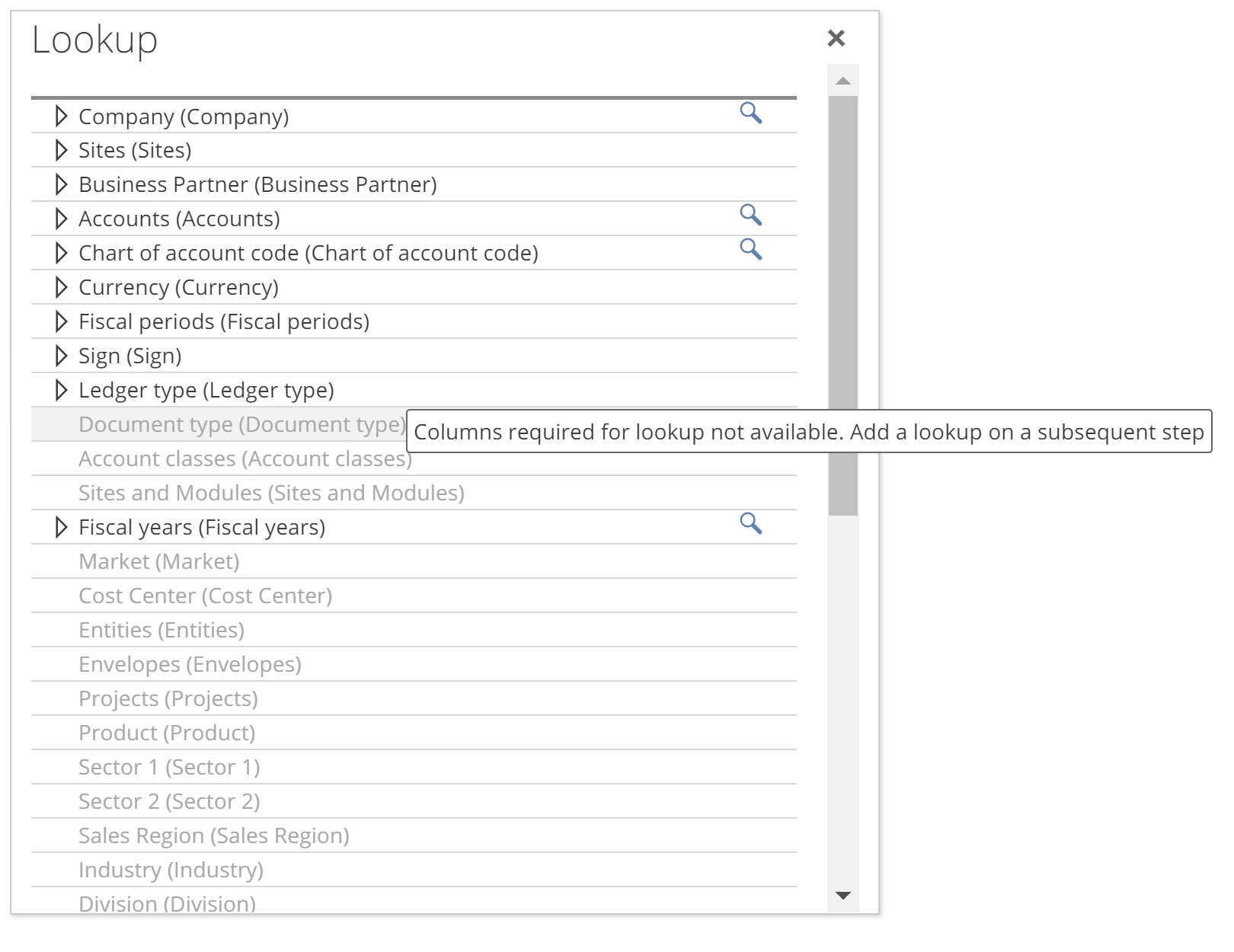 |
Why would that be? Let’s look at the relationship design panel for the Document type relationship to understand why we are unable to create a lookup from this Pipeline on the Initial Step.
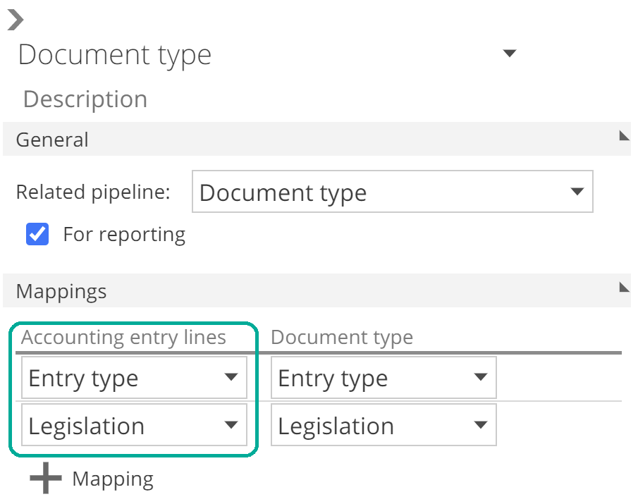 |
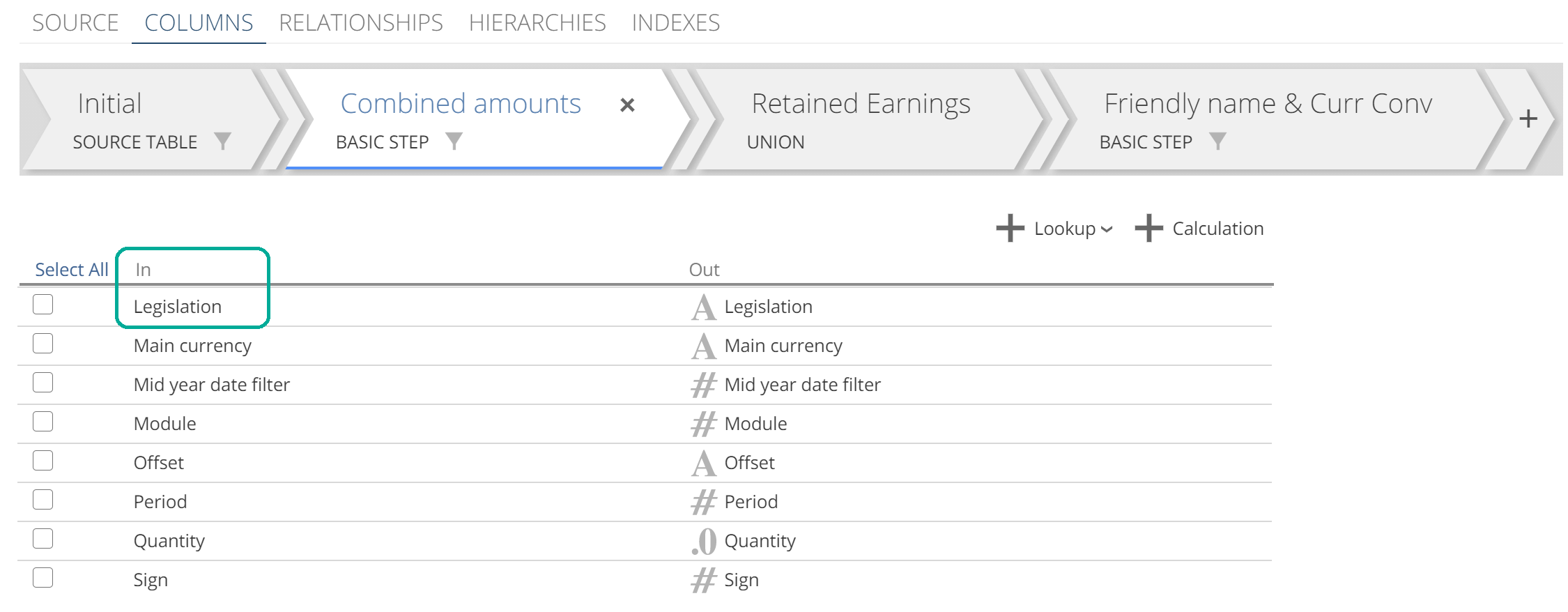
There are two columns required to relate the Accounting entry lines Pipeline to the Document type Pipeline. However, if we look at the Initial Step (on the COLUMNS tab), you can see that one of those columns (Legislation) is itself a lookup! This is identified by the magnifying glass icon, as in the following image.
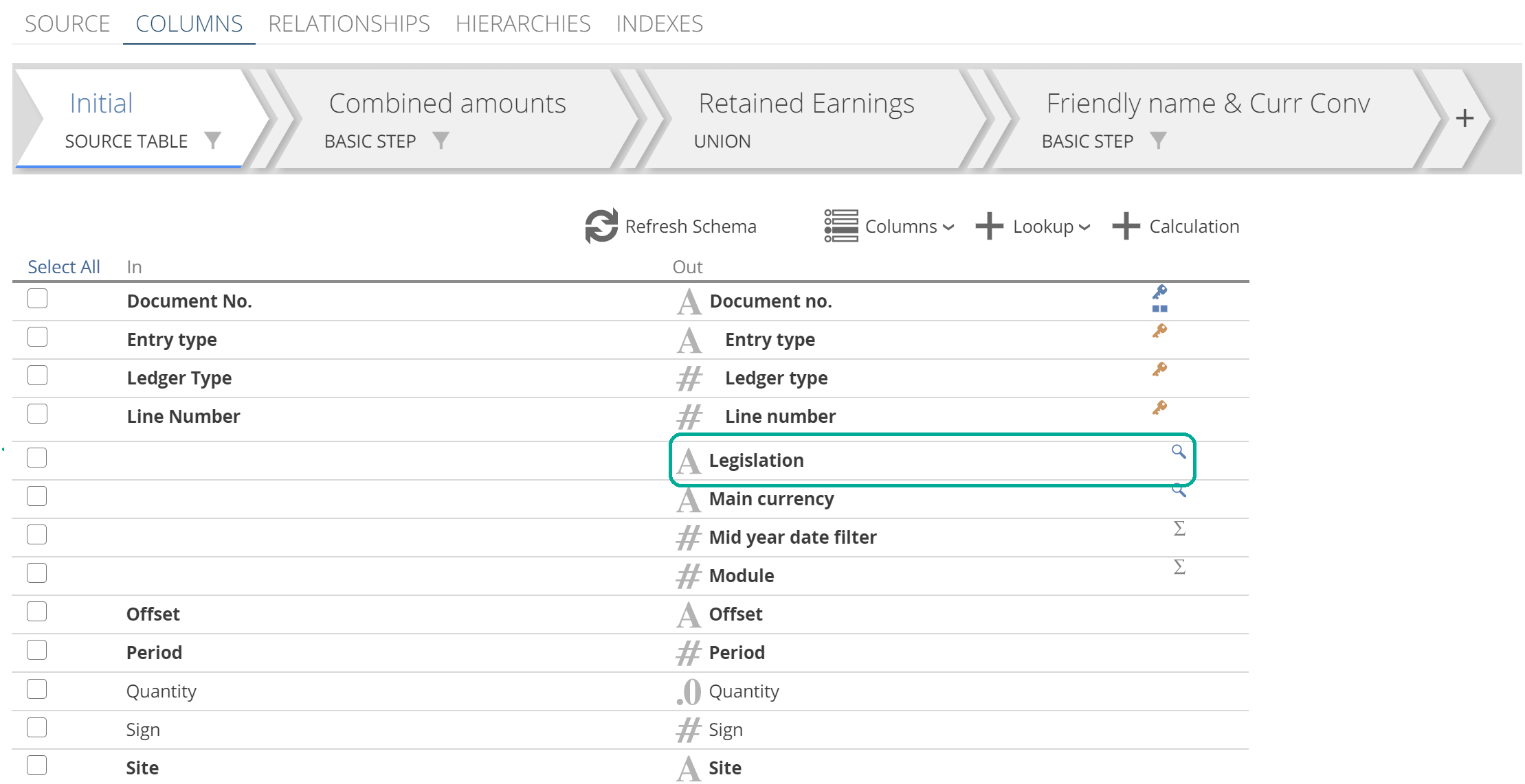 |
This is our first in-application example of the order of task views affecting the design of the Model. In this case, a lookup cannot make use of another lookup from the same step. It is subtle that a second lookup would make use of the Legislation lookup through the Document Type relationship. This is a slightly more complicated version of the example we saw where one calculation could not make use of another calculation from the same step. Shortly, we will look at how to follow the guidance Data Hub provided to address this issue, but first, we will close out our discussion of lookups.
Back to the Lookup pop-up, columns that are dimmed and italicized are associated with an existing lookup, as in the following image.
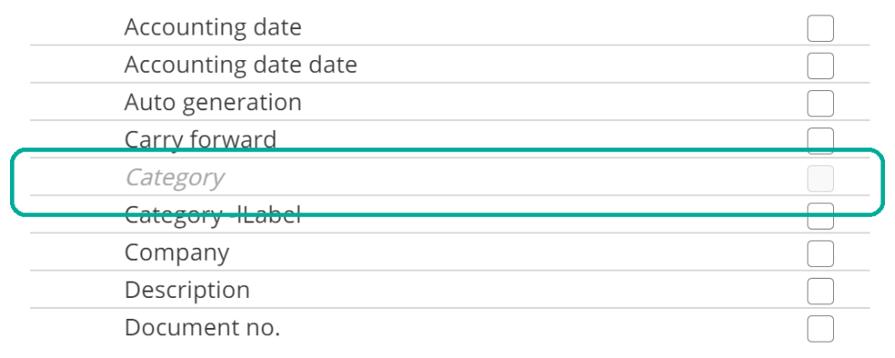 |
You remove a lookup column from the columns list by right-clicking the row and selecting Delete.
 |
Finally, you can navigate through multiple relationships to create a lookup. Again, after expanding a Pipeline, you see all columns for that Pipeline. In addition, you see all Pipelines that are related to that secondary Pipeline. If this is a little bit to take on, don’t worry, it’s all covered in a How-to, which you can refer to when you need (see Relate your pipelines).
Now, back to our previous issue. Recall that we were guided to add the Document type lookup on a subsequent step. Putting aside that this Solution pipeline already has a subsequent Step, how would we add a Step, and what Step type should we add?
Adding a Step
This will be quick. You add a Step by clicking on + from the Step tabs.
 |
You will be prompted for the Step type.
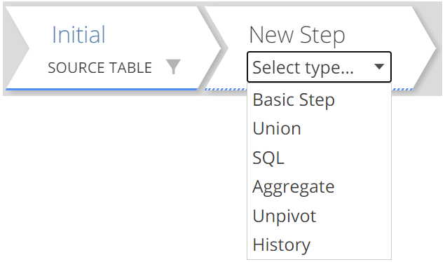 |
You can add a Step between existing Steps by hovering over the Step placeholder, as in the following image.
 |
Finally, should you need, you delete Steps by first selecting the Step, then clicking the small cross.
 |
The Basic Step
And now, for all but a few specific scenarios that we will address, the Basic step is the answer to the previous question. Namely, what Step type do we add? The primary purpose of the Basic step is to allow you to control the order of tasks (lookups, calculations, and filters). The Basic step does also serve a secondary purpose of allowing you to logically group these tasks, to improve the readability of your Pipelines.
We encountered our current issue on the Accounting Entry Lines Pipeline from the Data Hub Training solution. Previously we attempted to create a lookup on the Initial step. If we now select the second step (which is a Basic Step) and scroll down, you will see that Legislation does not have a magnifying glass because it is not a lookup on this Step. Moreover, from the In columns, you can see that Legislation flows into this step (this was not the case on the Initial Step). So we have values for Legislation even before the currents Step’s task views transform the data further.
 |
Given that Legislation is now available to us at the Step’s input (the set of In columns), we can use any relationship that requires this column. See it to believe it. Click on + Lookup. The Lookup pop-up shows, and it now allows us to expand Document type and select columns.
 |
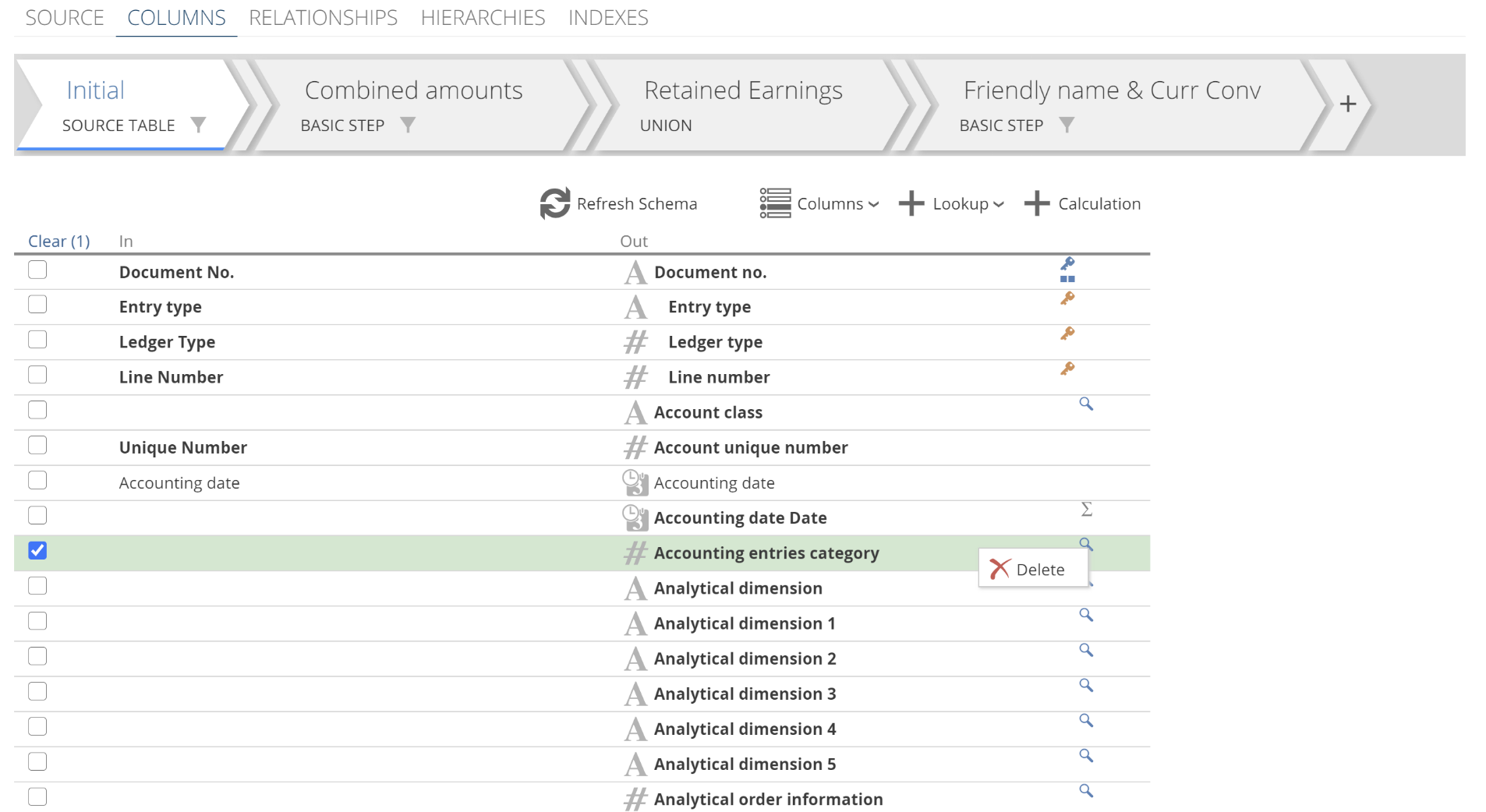
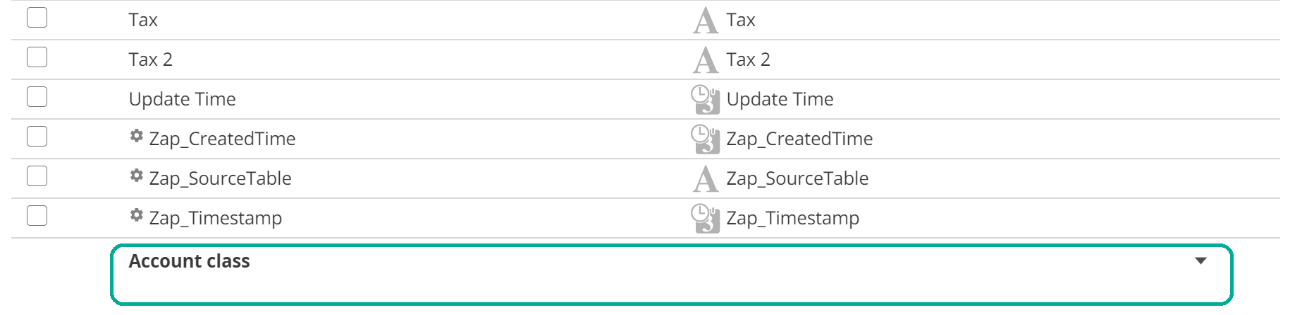
We just introduced the In columns in passing, and we have glossed over the following point until now. Each Step has a set of In columns and a set of Out columns. Each row on the columns list is a mapping of an In column to an Out column. You can right-click a row and select Delete, as in the following image. However, it is important to understand that this is only deleting the Out column. In the following image, the Out column for the Account class will be deleted.
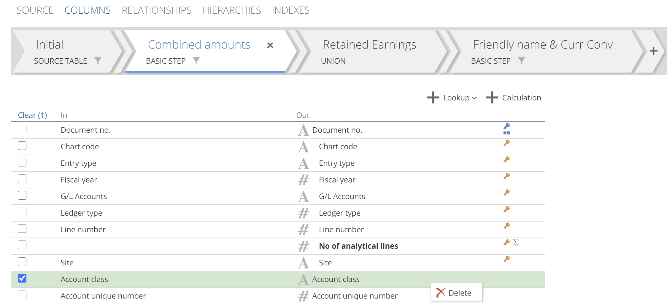 |
Having clicked Delete, if you now scroll to the bottom of the columns list, you will see that there is still an In column for Account class.
 |
By deleting the Out column for Account Class, we have unmapped for this and all subsequent Steps. From the image above, you can see that the Out column for Account Class provides a drop-down. This drop-down allows you to re-map the row to match the In column.
Unmapping represents a fourth task type that is performed after the three we have already introduced (lookup, calculate, filter). Because unmap is performed last, lookups, calculations, and filters can make use of any columns that are unmapped, on the same step.
Unmapping allows you to remove columns that have served their purpose on previous steps and are no longer necessary. It is best practice to remove such unnecessary columns to triage what the end-user sees in their analytic tool. Removing unnecessary Out columns also represents an important optimization tool for warehouse tables. Warehouse views are less impacted by unnecessary columns because their on-demand nature allows that extra columns to be ignored at query evaluation time.
Let’s cover off a few final points on the columns list while we’re here. If a column’s name or data type changes on a Step, its row will be bolded. If a column is new for a given Step (it is not included in the set of In columns), then it will also be bolded. Finally, if a column is unmapped on a given Step, it will again be bolded. You can see examples of these bolding rules in many of the images to come.
That is all there is to say about the Basic step.
Calculations
We have introduced lookups, with a quick foray into controlling the order of tasks with the Basic step. Now it is time to introduce calculations. To add a calculation, simply click + Calculation.
 |
This will result in a new column in the columns list. In the following image, we have jumped across to a Pipeline with fewer columns. We did this so that our new column does not get lost amongst other columns.
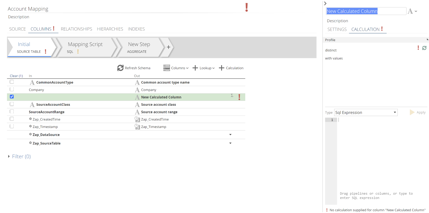 |
We will talk about the red exclamation marks shortly. The first thing to do is name your calculation. The default title text is already selected, so you need only start typing. Let’s leave the Type drop-down at SQL Expression for now.
You can drag Out columns from the columns list and drop them into the expression text editor. This saves you typing column names.
Additionally, if you start typing, autocomplete will offer you a list of options as in the following.
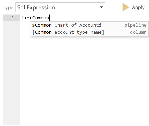 |
The example in the image is interesting because there are both a column and a Pipeline that start with the word “Common”. As this is a SQL expression, column names with spaces must be wrapped in square brackets. For this reason, if you enter an opening square bracket, and then type the initial characters of a column, autocomplete will only offer you a list of columns. Autocomplete provides the following item suggestion types:
Columns – columns from the current step. Type [ to filter to columns. While you can only drag Out columns from the columns list, you can still make use of columns that are unmapped on this step using autocomplete.
Pipelines – All Pipelines from the model. Type $ to filter to Pipelines.
Parameters – All Model parameters and all relevant data sources parameters. We will look at parameters in a future section. Type # to filter to parameters.
Step aliases – Allows an expression to reference the current task view. Type @ to filter to step aliases.
Keywords – SQL keywords. No prefix.
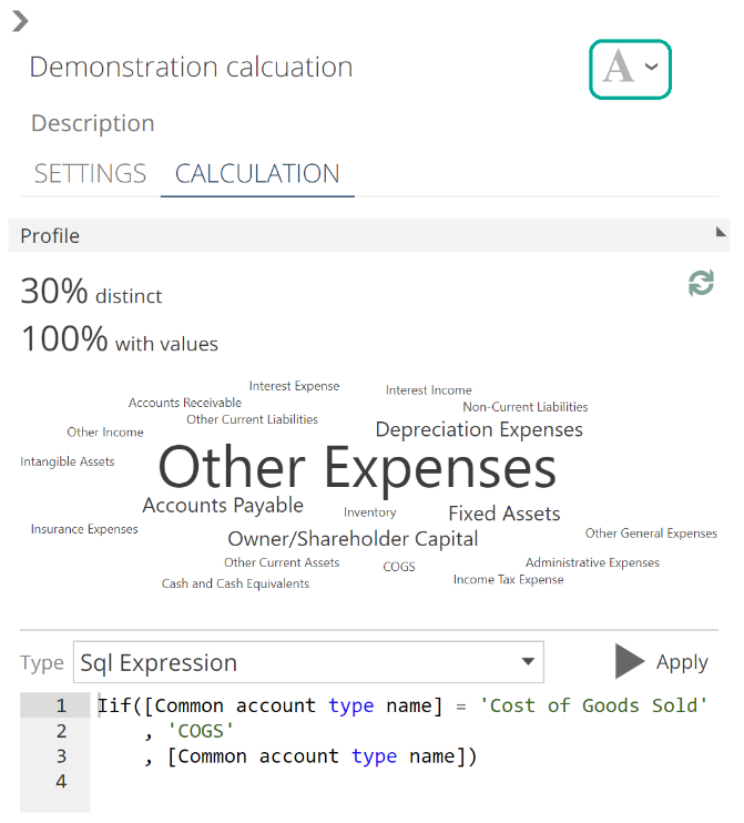
As you can see, you have all the tools to get very advanced. However, it is rarely necessary to define complex expressions. Data Hub has a suite of in-built calculation types to provide for most calculation requirements. We turn to these shortly, but first, specify your SQL expression and click Apply.
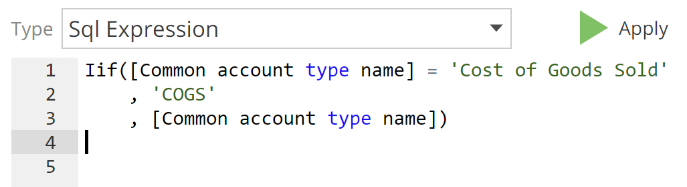 |
If the expression is invalid, a Model validation error will show against the expression as a red exclamation mark. Validation errors reflect up in the interface. That is, a column in error reflects as the Step being in error. The Step being in error reflects as the COLUMNS tab being in error. And finally, the COLUMNS tab being in error reflects as the Pipeline being in error. This is shown in the next image. The reason that validation reflects is to provide a trail of breadcrumbs for you to track down and resolve errors. You can see the details of the specific error by hovering over the red exclamation mark at any level (the Step-level in this case).
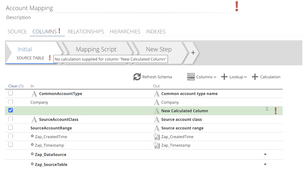 |
Let’s return to our task views. Recall that it is possible to create calculations based on lookups from the same step. It is not possible to create calculations based on other calculations from the same Step. These rules may become second nature in time, but until then, Model validation will tell you when you get it wrong. It is hard to ignore a big red exclamation mark.
And while we are at it, don’t ignore orange exclamation marks! Such exclamation marks are validation warnings. For example, It is possible to create a calculation without clicking Apply, and this will generate a validation warning. While the model may process with warnings, it is also quite likely to fail or perform very poorly. For this reason, do not leave validation warnings in production models. The How-to guide includes the Resolve common model validation warnings article (Coming Soon) as a resource to this end.
Now back to our calculation. If the expression is successfully validated, a profile of the calculation is shown immediately above it.
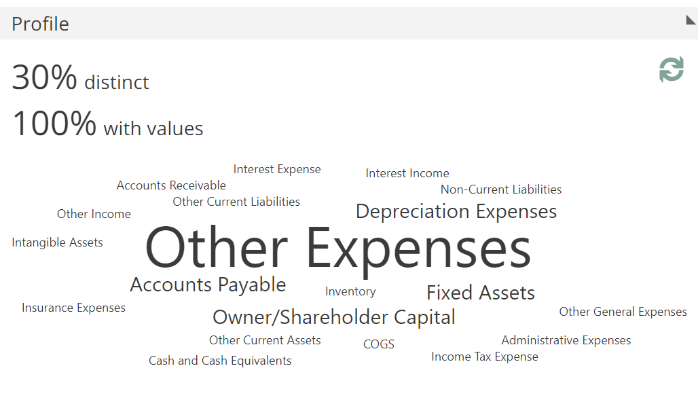 |
The data from this profile is used to configure the data type of the column.
 |
You can change the type. For example, to accommodate the additional length, as in the following.
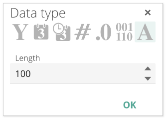 |
Don’t forget to click the OK button! And as usual, you can hover for more information on each type.
Let’s return to the Type drop-down. As discussed, Data Hub provides calculation types for many if not most calculation requirements. Calculation types are grouped by category, as in the following image.
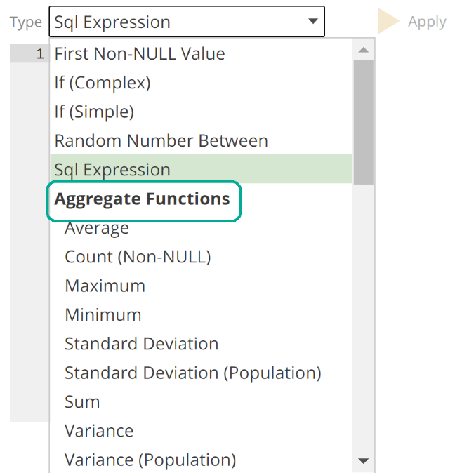 |
The available calculation types are grouped as follows:
Aggregate – For example, the Sum type would allow you to calculate the percentage that each order line represents within an order.
Analytic – For example, the Is First Value would allow you to determine if an order is the first for a given customer.
JSON – JSON functions allow you to manipulate JSON-structured columns from your source.
Ranking – For example, rank your customers by sales for a given period.
String – For example, concatenate First Name and Last Name columns.
Time – For example, the Difference Between Dates calculates the timespan between two date/time columns.
Let’s look at the Time example now. In the following, note that the Start and End column inputs are drop-downs.
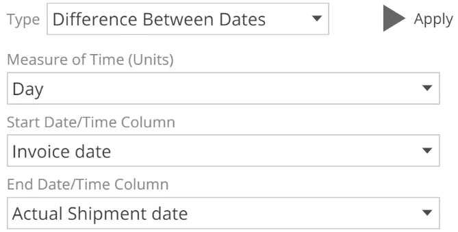 |
The calculation in this example can now automatically reflect name changes to these columns, by merit of them being specified with drop-downs. And if either column is removed, a validation error will show on this calculation. For comparison, a SQL Expression type calculation will not automatically reflect name changes, and it will only identify removed columns if the expression is re-validated (with the Apply button). In addition to these validation benefits, calculation types guide you down the path to optimal calculations. In particular, the Aggregate functions allow you to avoid certain expressions that can perform extremely poorly. For these reasons, it is best practice to use an appropriate calculation type where possible.
Often you will need to nest one calculation type inside another. This is performed by creating an inner calculation on one Step and an outer calculation on a subsequent Step. For very complex expressions this becomes cumbersome, and in this circumstance, you may elect to fall back to the SQL Expression type. However, keep in mind that there are very real benefits to using the purpose-built calculation types.
Common step features
Having previously introduced the Initial and Basic Steps, let’s discuss some capabilities common to all Step types. Recall we discussed the Filter section on the SOURCE tab. Filtering on the SOURCE tab reduces the volume of data that is loaded from the source into the warehouse. Each Step also has its Filter section. The interface of the Step Filter section is identical to that of the SOURCE tab. However, filtering on a Step only reduces the data volume that flows out of that step. Sensibly filtering on the SOURCE tab provides the greatest performance benefits, but there are two circumstances where it makes sense to filter on a Step:
The filter relies on columns that are not available in the source – This usually occurs when the filter is based on a lookup or calculation, that is, transformed columns. As alluded to previously, Data Hub does offer a solution to transforming the source data at extract time which would cater for source-filtering. This is performed with the Source SQL Pipeline, which we will see shortly. However, unless the benefit to source filtering is significant, it is best practice to rely on a Step filter in this scenario for Model maintainability.
The removed rows may serve a purpose in the future – And importantly, in this scenario, those rows might not be unavailable from the source in the future. If the rows are guaranteed to be available, it far better to re-load from the source as required. In this scenario, where the source rows might be unavailable, you will want to archive them with the History step. We will discuss the History step a little more in a future section.
Recall that to support filter building, the SOURCE tab’s Preview section provides a filtered preview of the source data. Each Step also has its own Preview section to provide a filtered preview of the data. The Step Preview table reflects the Out columns of that step. We did not see the Preview section last time, so let’s look at it now. At the bottom of the open Pipeline tab, click the chevron adjacent to the Preview heading. A preview of the data will now show.
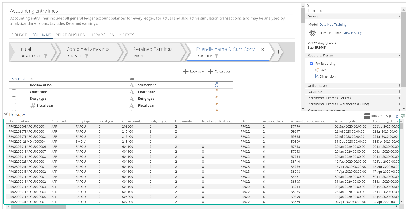 |
This preview may be based on sample data in which case the sample icon ( ) will show to the far left in the Preview toolbar. Sensibly there are limitations to sampled data, the details of which are available by hovering over the sample icon. The preview may also be based on the complete data set, as in the case of a processed model.
Either way, the preview is limited by the Row Limit specified on the Rows pop-up (click Rows to show the pop-up).
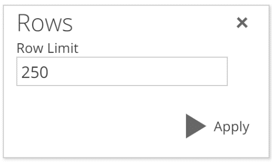 |
You can use the Download Preview Data option to download a CSV with the complete row set (not restricted to the Row Limit). However, keep in mind this complete row set may still be a sample. (again check for the icon) The Download Preview Data button is to the right of the SQL button. For Pipelines with many rows, and where the current step or previous steps introduce many lookups and calculations, the Download Preview Data may take some time.
The Preview section includes additional functionality for refreshing the sample against the source and investigating your data with SQL. We will not cover these topics here. When the time comes, hover over the buttons. You will be guided on how to use each of these features.
Parameters
At this point, we introduce parameters. Parameters are user-or-system-defined constants to improve the maintainability of your model and can be used in calculations, filters, and relationship mappings. Parameters can be specified on a Data Source and the Model. Data Source parameters are only available to those Pipelines using the Data Source. The parameters for a Data Source are listed on the PARAMETERS tab, as in the following image.
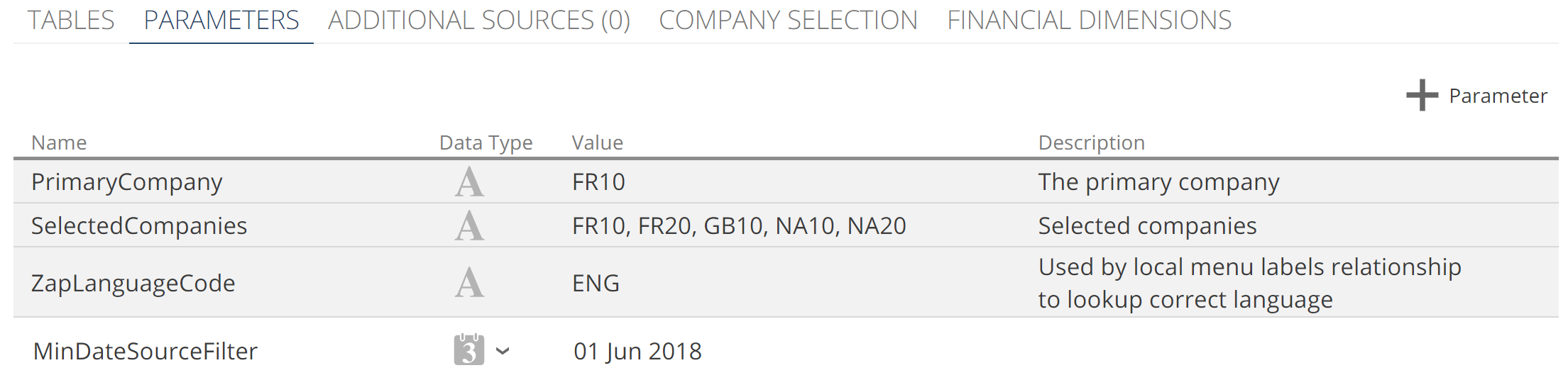 |
System-defined parameters are shown with a grey background. These parameters are created by Data Hub during the model creation wizard or based on the further configuration of the additional Data Source tabs (for example, COMPANY SELECTION and FINANCIAL DIMENSIONS in this image). Model parameters are defined in the PARAMETERS section of the Model tab.
Pipeline types and additional step types
We are now ready to close out our discussion of the modeling within Data Hub. To this point, we have only discussed Pipelines that source their data from a source table (recall we use table loosely to cover API endpoints, worksheets, etc.). It is also possible for one Pipeline to serve as the source of another. Such a pipeline is a Warehouse Pipeline. For reference, the Pipelines we’ve discussed now are Source Pipelines. There are two common reasons why you might use a Warehouse Pipeline:
Reuse – you have two different Pipelines that share many, but not all, of the same modeling requirements. In this case, it makes sense to perform much of the data modeling on a single master Pipeline. Two Warehouse Pipelines can then source their data from this master Pipeline.
Performance – similarly, you may have two different Pipelines based on the same large source table. In this case, it makes sense to only load the source data once. Two Warehouse Pipelines can source their data from the same Source Pipeline.
Admittedly these two points overlap somewhat, and there are a few different patterns that can be applied in each case. The Data Hub Cookbook (Coming Soon) provides more in-depth guidance on these data patterns and more.
Both Source Pipelines and Warehouse Pipelines provide an interface for selecting columns and filtering rows. However, on occasion, you require additional flexibility. Data Hub offers the Source SQL Pipeline for this purpose. The Source SQL Pipeline allows you to specify SQL that is run against the source. There are two key reasons why you might choose a Source SQL Pipeline:
Complex source filtering – On occasion, the columns required for filtering are not available in the source. We discussed this possibility when we introduced the reasons to use a Step filter over a filter defined on the SOURCE tab. And at the time we alluded to the Source SQL Pipeline as an alternative solution in this scenario. Again, keep in mind that unless the benefit to source filtering is significant, it is best practice to rely on a Step filter for Model maintainability.
Source summarization – in some circumstances, a very large source table may be summarized to reduce the amount of data loaded into the staging tables.
Having provided these two scenarios, it is important to point out what is being sacrificed when a Source SQL Pipeline is used. To start with, this is putting a load on the source. With source summarization, in particular, this load could be significant. Secondly, any changes to the source SQL query will require a full source data load. Finally, there are validation benefits to avoiding Source SQL Pipelines, in the same way, we saw benefits to avoiding the SQL Expression calculation type.
The following table summarizes the Pipeline types available:
Origin | Single Table | SQL |
|---|---|---|
Datasource | ||
Warehouse |
The Warehouse SQL Pipeline is new from this table. This Pipeline type provides a solution to complex in-warehouse transformations. It is rarely required due to the powerful transform Step types we will see shortly. We will not look at how to create each Pipeline type, because the concepts we have discussed cover all that you need to know, taken with the How-to section of the documentation. But if you have a hankering, you can take a quick look at the links from the table above.
It is also worth noting that the system-generated Date Pipeline is its own special type. The SOURCE tab of the Date Pipeline allows you to change the initial calendar configurations selected on the model creation wizard. More detail can be found in the Pipeline reference article.
In addition to different Pipeline types, there are additional Step types to discuss. You add these additional step types, as you would a Basic step, by selecting the appropriate type from the drop-down. As with most drop-downs, you can hover over each selection to get additional information. In the following image, you can see an example of particular rich in-application documentation.
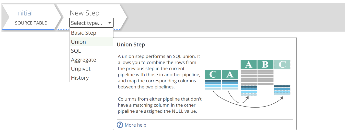 |
From the drop-down, you can see there are five Step types in addition to the Basic Step:
Union – combines the rows of one Pipeline with the rows of another. For example, as would be required to combine the Sales Orders tables of two different source systems. Although this represents a simple example, Data Hub provides more powerful options for combining sources as we will see later.
SQL – defines a custom transform in SQL. As with SQL Expression calculations and SQL Pipelines, this step type should be used very judiciously.
Aggregate – summarises or “aggregates” the Step’s rows. An aggregation type must be specified for each column. For example, a transaction pipeline with records down to the minute might be summarised to only include records down to the date. In this case, the aggregation type for the Amount column would be Sum, and the aggregation type for the Date column would be Group. The remaining columns would most likely also use either the Sum or Group aggregation type. Additionally, the Aggregate Pipeline can be used to remove duplicate rows. We will address duplicate rows in a little more detail when we return to the topic of keys. With this high-level explanation in mind, you can refer to the How-to documentation when you see a need to summarise or remove duplicates from a Pipeline.
Unpivot – transforms pivoted source tables, usually from Excel and CSV documents. We will leave it at that, and the hover-documentation will guide you when the time comes.
History – allows you to identify source data changes and also archive source data rows that would otherwise be unavailable at a future date.
Let’s just quickly expand on the History step, because the ability to capture historical data is a significant benefit of data warehouses. Take an example where the source system provides sales opportunities but does not track changes to the sales opportunity values, as is most often the case. The History step would allow you to track those changes to sales opportunities and more accurately forecast your actual sales. The Opportunity Pipeline would include a History step, and it would be configured to process regularly. On each of those regular processes, the History step would compare the current data from the source to the previously captured data in the warehouse. If a value that was being tracked changed, the History step would capture that change in the warehouse.
The History step can also be used to archive source data. Many source systems provide only a limited window of data. For example, an API providing health metrics for a service might only provide 30 days of data. To identify longer-term trends, older data must be archived. The History step offers a solution to archiving this data in the warehouse.
In both the change-capture and archive scenarios, the data warehouse becomes the sole source of truth. This is important because it has backup implications if you are not running in ZAP Cloud. There is a lot more that can be said of the History step and all the Step types above. However, by now we have addressed all the concepts you will need to know. So when it comes time to use one of the additional step types, you will be able to work with the in-application documentation (available on hover) or work through one of the How-tos from the documentation.
At this point, we’ve loaded and modeled our data. There are a few more concepts to round out this article, but we’re getting close.
Processing and publishing
The Process pop-up
Recall that, after completing the Model creation wizard, we clicked Process Model on the Model tab to show the Process pop-up. Let’s now look at the options from that pop-up.
 |
Starting with the Publish changes checkbox, it is important to understand that there are two copies of a model at any time:
The design Model – is what you see in Data Hub.
The published Model – is a snapshot of the last design Model to be published. A design Model is published if Publish changes is checked, and the Update warehouse structure step from the Process tree is successful. We will expand on this shortly. If Process Warehouse is checked on the pop-up, the design Model must also successfully process.
Keep in mind that the Model is only a high-level plan for the warehouse, and it is not the warehouse itself. There is only ever one warehouse and therefore only ever one copy of the data.
The published Model is used for all scheduled Model processing. This allows you to work on the design Model (again what you see in Data Hub) without affecting scheduled data refreshes. However, keep in mind that if you observe an error during a scheduled Model process, that error is with the published Model, which is not necessarily in synch with the design Model.
The Publish changes checkbox is checked by default if there are changes to publish. A summary of these changes will show below the checkbox, and the Show Changes option will show, as in the following image.
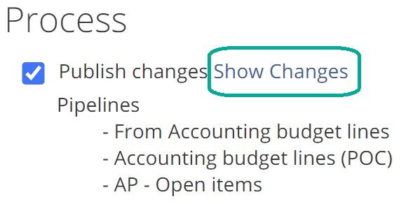 |
Clicking on Show Changes will open a new tab showing the differences between the design Model and the published Model.
As a quick aside, from the Introduction to Data Hub article (Coming Soon), you may recall that it is possible to compare any two resources of the same type. In this scenario, Data Hub is comparing two Model resources (the design Model and the published Model). It is also possible to compare an under-development Model to a production Model, or the production Model to a historic copy of that model. These are very powerful capabilities to keep in mind for managing the lifecycle of your Model. The Compare resources how-to provides further guidance on this topic.
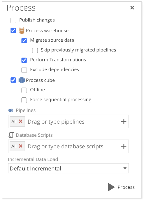
Returning to the pop-up, if the Process warehouse checkbox is checked, you must also check at least one of the following:
Load source data – the model process will load source data into the staging tables.
Perform transformations – the model process will transform the data by migrating it from staging tables to warehouse tables for any materialized pipelines.
Also under the Process warehouse checkbox is the Exclude dependencies checkbox. This checkbox allows you to skip processing the dependencies of the specified Pipelines and scripts. We will talk to dependencies shortly. We will not, however, cover the Process cube options from this pop-up. These options are discussed in the Complete Guide to the Semantic Layer article (Coming Soon).
So we turn to the Pipelines and Database Scripts fields. These fields allow you to configure a subset of Pipelines and scripts to be included in this Model process. You can drag Pipelines from the Model tab’s Pipelines list or start typing a Pipeline name. Model scripts are beyond the scope of this document, and they are rarely required in a well-considered Model. However, if you are familiar with database scripts, be aware that this capability exists and you may refer to the documentation as needed.
And now, returning to the dependencies we alluded to earlier, Pipeline dependencies can be found on the Pipeline design panel. The following image shows the dependencies (Uses) and dependants (Used By) of the Accounts Pipeline.
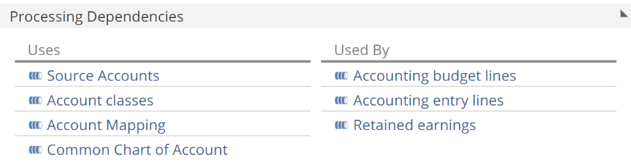 |
The primary source of dependencies (Uses column) is lookups. However, a Union step, a SQL step, or a SQL Expression calculation can also introduce dependencies. Sensibly the source Pipeline of a Warehouse Pipeline is also a dependency.
Finally, the Incremental Data drop-down allows you to specify the incremental processing behavior of each Pipeline. We will discuss the options for this drop-down in the Optimize section. For now, the Default Incremental option should suffice.
The Process tree
Having clicked the Process button on the Process pop-up, the process tree will show in the Model design panel. Following is a Process tree for a completed process.
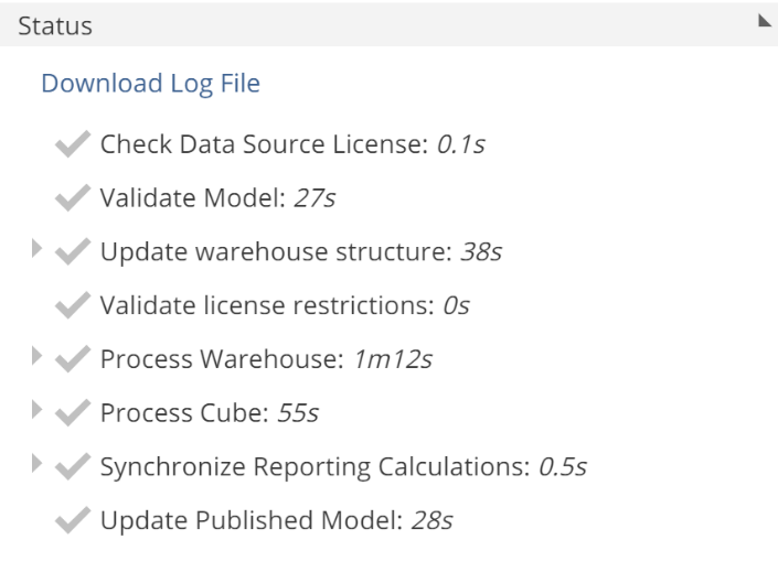 |
Let’s quickly discuss each of the non-licensing steps:
Validate model – the Model is assessed for validation errors. Any validation errors will cause the Model process to fail at this step.
Update warehouse structure – if Publish changes was checked, the warehouse structure is updated to reflect the current design Model. This step also ensures the warehouse structure is synchronized with the Model, even if Publish changes was not checked. If this step fails, all changes are reverted. If any subsequent step fails, an additional Update warehouse structure step will show on the tree, again, to reflect all changes being reverted.
Process warehouse – both source and warehouse processing is performed.
Process cube – the semantic layer is processed. For more information, see the Complete Guide to the Semantic Layer (Coming Soon).
Update published model – if all previous steps are successful, the model is published. That is, the published Model is updated to be a snapshot of the current design model.
During Model processing, some of the nodes we discussed above expand to show Pipeline-level detail, as in the following image.
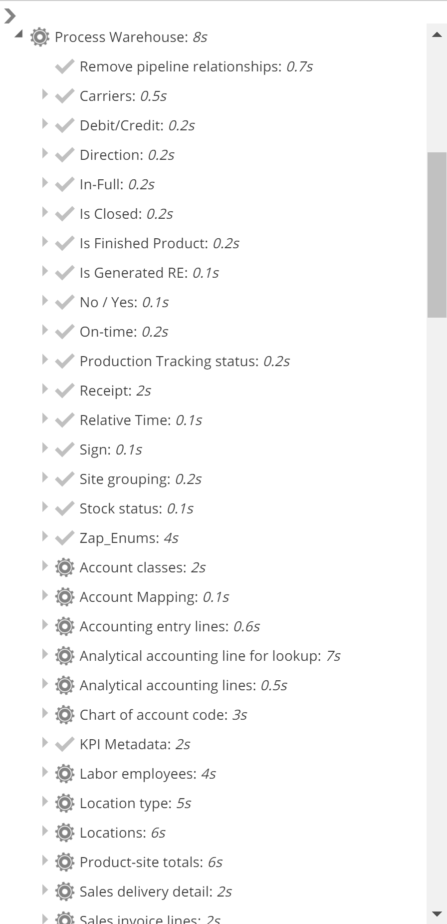 |
The timings shown allow you to identify the slower Pipelines in a Model process. It is also possible to expand Pipeline tree nodes to see source-load and transform operation timings, amongst other detail.
If there is an error processing (or publishing) a specific Pipeline, it will show on the process tree, as in the following image.
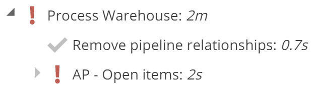 |
And as usual, you can hover over the exclamation mark for detail on the error. There are six categories of errors you may encounter, which we will discuss when we cover the Background Tasks tab. You can also expand the tree to see the error in context at a lower level.
At this point, we have a comprehensive understanding of both processing and publishing. It is time to provide some guidance on how best to combine the two:
Publish only – You may choose to publish only (uncheck Process Warehouse on the pop-up) when the structural change may be expensive (due to key or index changes). In this scenario, you don’t want a subsequent source-or-warehouse processing failure to revert the change.
Publish and process – This is the default option from the Process pop-up. Choose this option when you want your design Model changes applied, but reverted should the Model process fail for any reason.
Process only – You may choose to process only (uncheck Publish changes) when you want to ignore your current design Model changes and manually refresh the data for the existing published Model.
We can now close out our discussion of processing and publishing with a few easy topics.
Process Configurations
Process Configurations allow you to process a given set of Pipelines and scripts, with a given set of options, on a schedule or interval. You add Process Configurations with the + Process Configuration button from the Process Configurations section of the model resource. This is shown in the following image.
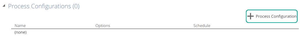 |
Once you add a Process Configuration, you configure it in the design panel to the right. The processing options are as we saw on the Process pop-up. The key difference is a new Schedule section, as in the following image.
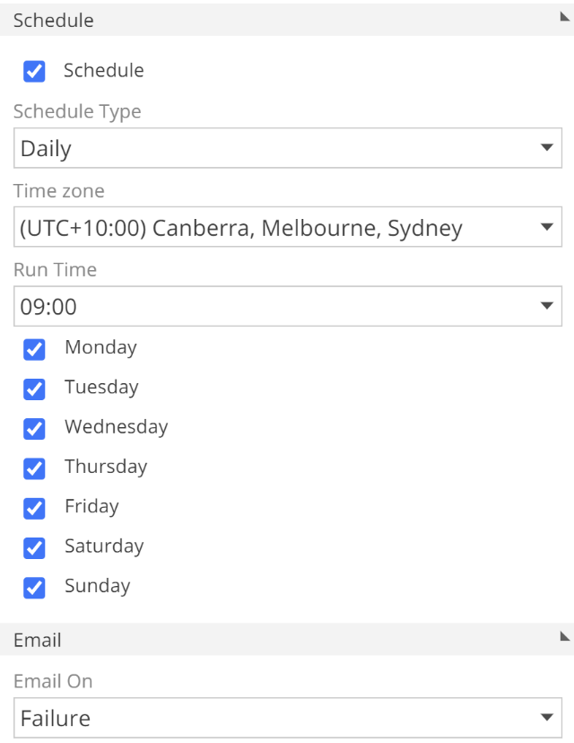 |
The in-application tooltips provide more information on each of these scheduling options. There is one more configuration option to note, the Email On drop-down.
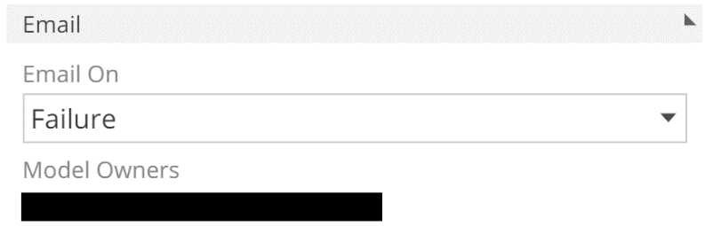 |
The Model Owners are configured in the Model design panel (de-select the Process Configuration to show), as in the following image.
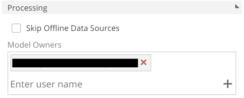 |
This setting is very useful for alerting on failure (the default behavior). It can also be very useful to notify you when a Model process completes successfully. We will talk to the Skip Offline Data Sources option shortly.
Background Tasks tab
The Background Tasks tab is accessed from the Settings menu (small cog to the top right) and provides a 28-day history of all Model processing tasks. It also includes a history of some analytics-related tasks that we won’t talk about in this article. History can be filtered by clicking on a specific resource from the Resources list (the panel on the left), or with the Date drop-down. The following image shows the Background Tasks tab filtered for the Data Hub Training Solution and the last 24 hours.
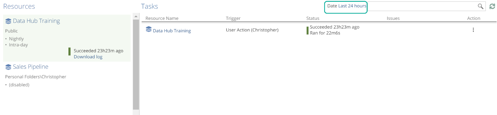 |
You can search by resource name and refresh the Tasks list with the options from the top-right, as in the following image.
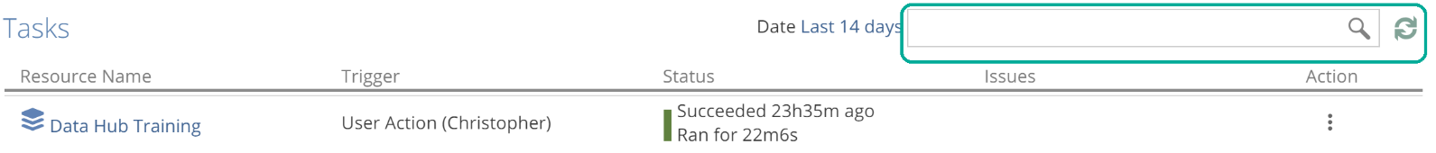 |
The Background Tasks tab also allows you to see the enabled Process Configurations for each Model resource, and a micro-chart of the most recent run-times.
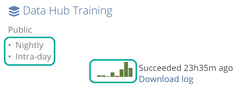 |
This information is important for managing the load on your systems.
If a model process fails for whatever reason the Issues column provides an error category.
 |
There are six error categories to be aware of:
Data – Data has violated the expectations of the Model. For example, source data not matching the data type specified on the Pipeline.
Environment– An environmental error has occurred. If you are using ZAP Cloud, be assured we’re already on it!
Gateway – The Data Gateway is offline.
Model – There are validation errors present in the Model, or a data source schema has been updated, and this change cannot be reconciled with the current Model. Common examples include invalid SQL in a SQL Expression calculation, and a column having been removed from a source system.
Source – There was an error with one of the source systems, or a required source system is unavailable.
Unexpected – Well, we weren’t expecting that. Please contact the support team.
And now to tie off another thread, let’s quickly refer back to the Skip Offline Data Sources checkbox that we saw on the Model design panel. This checkbox allows Source-category errors to be instead treated as warnings. By selecting this, Model processing will skip source-loading for Pipelines that would otherwise provide a Source category error. And the Background Tasks list would instead show a warning icon for the Model process in question.
Back to our image, and you can hover over the error category from the Issues column for a detailed description of the problem and the resolution steps.
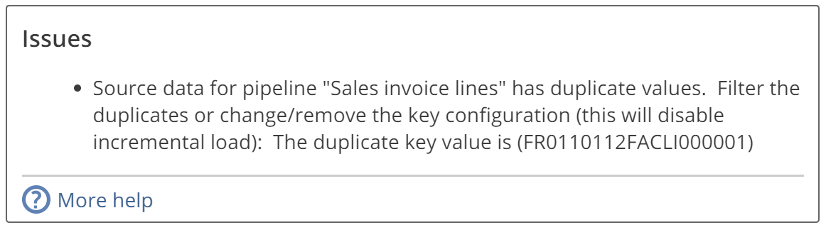 |
While this information is usually enough to solve most issues, the Troubleshoot a failed model process article (Coming Soon) provides additional guidance should you need it.
And finally, there are actions available from the Action column of the Task list.
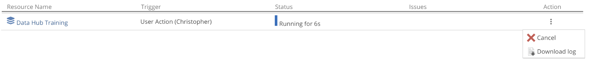 |
You may choose to cancel a running Model process to free up resources for other tasks. Download Log provides a very granular log of the Model process, including the SQL queries executed against the warehouse. This log may be useful for advanced users, and the Support team may request that you provide this log to aid in problem diagnosis.
Optimize
The big hitters
Let’s assume that you’ve already made sensible decisions about what data to load into your warehouse. That is, you have not brought in 15 years of data and included every source column (unless this was an explicit requirement of your business). We can now discuss at a high level how you would optimize your Model. For this, we do need a little theory.
To start with, some quick revision. Recall that the warehouse schema holds the tables and views for end-user reporting. Each Pipeline has either:
A warehouse table that holds transformed data as a result of querying the final staging view,
or a warehouse view that is a direct query of that final staging view. Again, such views provide an on-demand transform option.
We refer to the generation of a warehouse table as materializing the Pipeline. The model designer configures whether or not each Pipeline is materialized. We previously alluded to the fact that there are performance and storage considerations to choosing between warehouse tables and warehouse views. It is time to tie off this thread.
The vast majority of optimization comes down to the following, on a per Pipeline basis:
Configure incremental source processing – Ensure incremental source processing is appropriately configured wherever possible.
Appropriately select between warehouse table and warehouse view– If a warehouse table is used, ensure incremental warehouse processing is appropriately configured. We will discuss incremental warehouse processing next.
Ensure no warnings are present – Remove even those warnings that do not relate to performance, as they may obscure future performance warnings.
Further performance guidance can be found in the Modeling Performance Guide and the Troubleshoot processing performance article (Coming Soon). However, if you keep the previous three points in mind, you may find little need to refer to these articles.
We have already spoken to incremental source processing. We will not go over this again, but please note that this item was first on our optimization list. Warnings will always provide explicit guidance on how they should be resolved and the Resolve common model validation warnings article provides additional guidance, should you need it. Finally, you will get a chance to practice resolving performance warnings with the practice problems linked from the bottom of this article.
Warehouse tables and incremental warehouse processing
So we turn to the decision between warehouse tables and warehouse views. Let’s talk to the benefits of each:
Warehouse tables – perform expensive transforms once, either on the initial full migration or on a subsequent incremental migration (for added or update rows). This assumes that incremental warehouse processing is configured.
Warehouse views – avoid the cost of populating a warehouse table by performing transforms on demand.
A quick aside, we noted in the architecture section that there are additional storage considerations to warehouse tables (keep in mind that all data is first loaded into staging tables). Importantly, this additional storage is not considered for licensing purposes.
Time to provide some basic heuristics on when to use either a table or a view:
For trivial Pipelines, create views – A trivialPipeline is one that includes only an Initial Step and optionally source and Step filters, but importantly no calculations or lookups. Trivial Pipelines of any size should result in warehouse views.
For all other Pipelines, create tables – Pipelines that do not conform to the previous definition of trivial, should result in warehouse tables. Often it is not the Pipeline itself that benefits from this configuration, but rather a dependent pipeline.
For very large simple Pipelines, experiment with views, as required – Occasionally for very large, simple Pipelines (>10M rows), on-demand performance is good enough that the expense of a full migration is not justified. Following the previous two points, you will have already configured this Pipeline to result in a warehouse table. As an exercise in optimization, you may experiment with configuring the Pipeline to generate a warehouse view Instead.
Having provided these heuristics, keep in mind that if you created your model from a Solution, these Pipelines come preconfigured for optimal processing in most environments. In addition to this, validation warnings may guide your decisions to materialize in some circumstances. So, it is possible to build many if not most small-to-medium Models without paying any attention to the decision to materialize.
Now, once a Pipeline is configured to generate a warehouse table, and after the initial full load, only the added and (optionally) updated rows should ever be migrated from the staging table. That is, we want to ensure incremental warehouse processing is configured. And here is the challenge for larger Pipelines. The cost of incrementally processing the rows can be considerable depending on the transforms on the Pipeline. At the extreme, it can more than offset the inherent benefits of materializing a Pipeline, resulting in slower overall performance. This should provide some justification for why it is occasionally necessary to fall back to a warehouse view.
Incremental warehouse processing requires keys on the warehouse table so that the rows to be updated can be uniquely identified. That is enough theory, let’s return to the application and start by ensuring warehouse table keys are in place.
The following image shows the Sales order lines Pipeline from the Data Hub Training solution. It has been slightly modified for the purposes of this example.
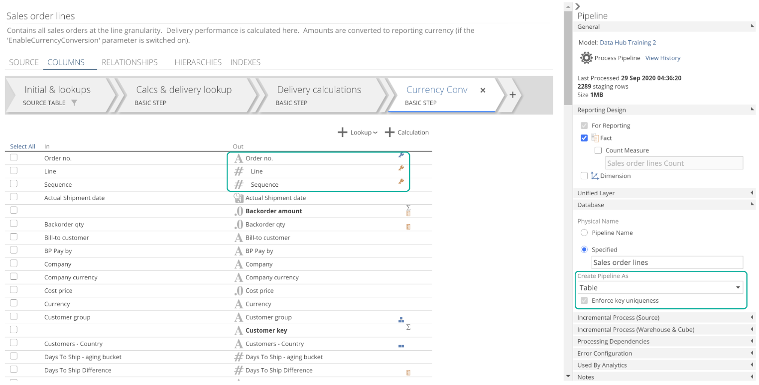 |
The first thing to note is the Create Pipeline As setting. This is where we choose between a warehouse table and a warehouse view. In this case, we have set it to Table because we, for example, added an onerous calculation on a previous step. Also, note that this image is showing the keys for the final Step of the Pipeline. Pipeline keys on the final step provide the keys for the warehouse table (if any). Again, incremental warehouse processing requires these keys. And we saw previously that Pipeline keys on the Initial step provide the keys for the staging table. Importantly, Pipeline keys on the Initial step and the final step can be configured independently, as can data types for that matter. The keys should, however, only differ if a non-Basic step used. For example, a Union step may justify keys changing between the Initial and final Step.
With final-step keys in place, it is time to configure this Pipeline for incremental warehouse processing. Expand the Increment Process (Warehouse & Cube) section from the Pipeline design panel. First, ensure that Warehouse Incremental Load is checked.
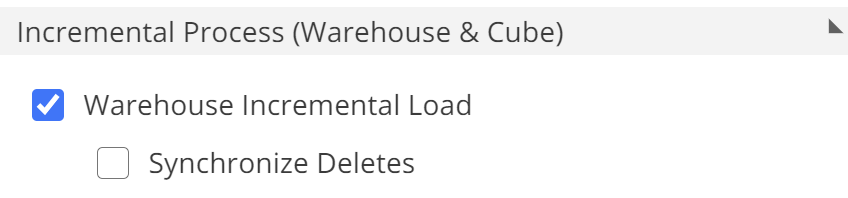 |
A quick side note, cube processing is discussed in the Complete Guide to the Semantic Layer article (Coming Soon).
If data can be deleted from the source table and these deletions are relevant to your reporting requirements, you may check Synchronize Deletes. This synchronizes deletions between the staging and warehouse tables, but with a performance penalty. Synchronize Deletes is generally useful for API-sourced or spreadsheet-sourced Pipelines that are subject to deletions, and where Data Hub has directed you to materialize for performance reasons. Should you be interested, the details on why Data Hub may direct you to materialize in some circumstances can be found in the Modeling Performance Guide (Coming Soon).
Moving on, for the sake of this example, check Override settings from data source. As with incremental source loading, we can configure incremental warehouse defaults on the data source, but we will quickly cover that later.
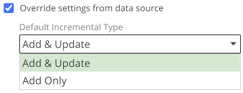 |
There are two different incremental warehouse load behaviors:
Add & Update – rows that have been added or updated in the staging table are migrated to the warehouse table.
Add Only – only rows that have been added are migrated to the warehouse table.
Incremental source processing does not provide the Add Only option. That is, incremental source processing will always load all added or updated rows. Incremental warehouse processing provides this degree of configurability because Add Only warehouse processing can perform significantly faster than Add & Update. The differences are as follows:
Add Only – processing need only add new rows from the Pipeline’s staging table (based on the staging table’s system Zap_CreatedTime column).
Add & Update – processing must add rows using the same logic as Add Only. Processing must also update rows (based on the staging table’s system Zap_Timestamp column) and check if any lookup columns have in turn been updated. Sensibly for a Pipeline with lookups from many different Pipelines, this last step can be expensive.
In the event of a source full refresh or structure changes to the Pipeline, neither incremental type applies because a full warehouse refresh is required.
We have seen the two incremental load behaviors. There are also two different incremental types: Default and Quick.
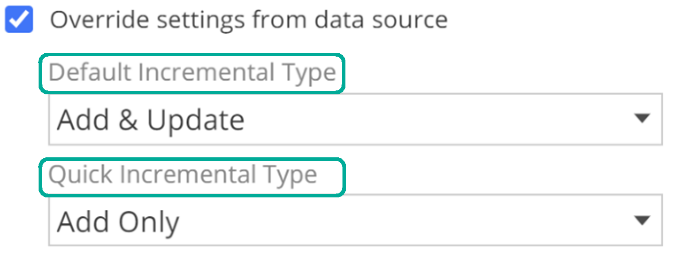 |
These are just categories for convenience. The combination of incremental process behaviors and incremental process types allows the designer to specify the behavior at the Pipeline level and choose which Model-wide type to apply at process time.
It’s time for some guidance on how to configure Pipeline incremental behaviors for each type. Let’s start with the ideal scenario in which we refresh all data on the desired schedule, with no concessions to performance. This configuration requires configuring incremental behaviors for only the Default Incrementaltype. Each Pipeline’s Default Incrementaltype drop-down should be set as follows:
Transaction Pipelines set to Add Only – Transaction Pipelines are those where each row captures a movement of an entity (for example inventory or currency). This movement represents a transaction. It is generally accepted best practice that transactions are never deleted, even in the case of errors. This practice ensures an audit trail. For example, an Inventory Transactions Pipeline would represent a transaction Pipeline.
Snapshot Pipelines set to Add and Update – Snapshot Pipelines are those that capture (or snapshot) only the current state of a business entity. For example, a Sales Order or a Sales Order Line Pipeline would represent a snapshot Pipeline.
Descriptive Pipelines set to Add and update – descriptive Pipelines are those that serve only to describe transaction or snapshot Pipeline values and hold no values of their own. For example, a Customer Pipeline would represent a descriptive Pipeline.
In the scenario just described, the Model is scheduled to process only the Default Incremental type, and on whatever schedule is required.
For large or complex models, processing may take a considerable amount of time. This may limit the frequency at which the model can be processed. It is also worth noting that ZAP Cloud Model processing times should fit within the guidelines of the ZAP Fair Use Policy. So, let’s take the scenario where the Default Incrementaltype cannot process within the required time (and let’s assume this model has already been fully optimized). The following should be configured:
Default Incremental type – Each Pipeline’s Default Incremental type drop-down should be configured as in the previous scenario. A Default Incremental Model process should be performed nightly or weekly.
Quick Incrementaltype – Snapshot or descriptive Pipelines that are slow to process can be set to Add Only. This configuration makes some concessions to data recency to improve processing performance. For example, a Sales Order Lines Pipeline configured for Add Only will process faster, but may not reflect an updated amount or customer detail until the next Default Incrementalprocess is performed. The Quick Incremental type Model process could be performed intra-day or nightly.
We will see shortly where individual Pipeline process times are reported in the interface, to help guide the above decisions. In the same section, we will introduce how processing is scheduled. Keep in mind that all of the above guidance applies to incremental warehouse processing. Incremental source processing generally represents less of a performance concern. However, in the case where incremental source processing is not configured, or a full refresh of source data is performed, the warehouse tables are necessarily also processed in full.
We strongly recommend that you do not schedule regular full refreshes. The configurations above should provide complete data accuracy, with some concessions to recency where required. A scheduled full refresh would imply data quality issues that are not fully understood. Such issues should be investigated and resolved, with aid from the Troubleshooting section of the Modeling How-to where required. If a subset of Pipelines requires full refreshes due to deletions that are relevant to reporting, and there is no solution to configuring incremental source processing for these Pipelines, then a separate processing schedule should be configured for only this subset. For models with a large amount of data, a full load introduces the risk that having dropped all data, one or more of the data sources subsequently go offline. This would leave the warehouse in an unreportable state.
Indexes
To close out our discussion of performance, we will now discuss indexes. An index is an “address book” for a given table, and a table can have multiple of these address books. Indexes make it quicker to find rows. For example, take a Customer table and imagine you are seeking a particular row for a given customer name. Instead of searching the table top-to-bottom, you could refer to an alphabetically-ordered index and have it tell you exactly where in memory the row exists. Indexes are created on the INDEX tab. Click + Index to add an index, like the following.
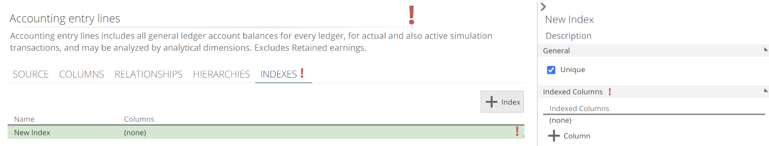 |
We see the now-familiar validation errors because we have yet not specified Indexed Columns for our index.
Click + Column to add one or more index columns.
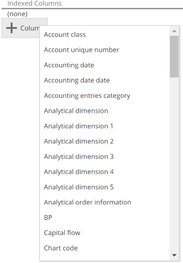 |
Adding indexes for performance is an advanced optimization technique and is generally only applicable to very large warehouses. For more information on when an index may be applicable, see the Modeling Performance Guide (Coming Soon). It is worth noting that Data Hub always generates the following implicit indexes to optimize processing:
Initial and final step key-indexes – Initial Step keys result in a matching index on the staging table. Final Step keys result in a matching index on the warehouse table (if any).
Incremental Add indexes – The Zap_CreatedTime columns of staging and warehouse tables are indexed to optimize incrementally adding rows.
Incremental Update indexes – The Zap_Timestamp columns of staging and warehouse tables are indexed to optimize incrementally updating rows.
Indexes perform a secondary purpose, and that is to aid in the prevention of duplicated rows. This leads us nicely to data validation.
Data validation
Data validation is the process of ensuring the numbers are correct. If during data validation, a data error is identified, then the next task is to diagnose the issue, wherein the root cause of the data error is investigated. Issue diagnosis and resolution are beyond the scope of this article. They are, however, comprehensively covered in the Troubleshoot wrong numbers in the warehouse article. By using a Solution Model as the basis for your design, the requirement for validation and diagnosis is significantly reduced. Nonetheless, it is essential to perform data validation on all Models, including Solution Models. While the Model deployment process is simple, there are still options that can be misconfigured.
Data validation is performed automatically by making use of Data Hub features. Additional data validation should then be performed manually by comparing reporting data to source reports. We turn to automatic validation first.
Automatic data validation
Data Hub provides two familiar tools for automatic data validation, namely keys and indexes. Both keys and indexes cause model processing to fail in the event of a data validation error, and this is desirable. These tools identify data validation errors with certainty. By preventing the Model process from completing, Data Hub ensures it is not possible to report on invalid data. Recall from the Process Configuration section that you can be alerted in the event of a Model process failure.
In addition to validation errors, Data Hub also provides validation warnings where there is a reasonable probability of invalid data. We covered validation warnings previously. To reiterate, Model validation warnings should be addressed before a Model is used in production. Let’s now discuss the use of keys for data validation.
Keys for data validation
As we have seen, keys serve the two essential purposes of supporting incremental source processing and supporting incremental warehouse processing. Let’s now discuss a third, equally important purpose. Pipeline keys also enforce that unintended duplicate rows are not introduced during modeling. Importantly they enforce this for both warehouse tables and warehouse views (with a validation query). As you can imagine, unintended duplicate rows almost guarantee that your numbers are wrong. Fortunately, Data Hub can equally guarantee that you will not introduce duplicate rows during modeling if all your Pipelines have logically correct keys and if all validation warnings are resolved. It is still possible that duplicated rows exist within the source system. Pipeline Keys will not protect against source duplicates which is why it is important to use high-quality data sources or de-duplicate your source data in advance of modeling.
Let’s first see an example of duplicate rows, to put us in the position to discuss the importance of the keys being logically correct. Take the following preview of a Customers Pipeline, which is the result of combining a legacy sales source with a new sales source. Sensibly most customers exist in both sources.
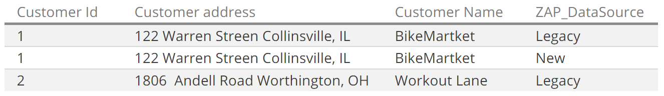 |
The duplicates here are obvious. Assuming the key for the Customers pipeline is currently Customer Id, this Model will fail at processing time (again this is desirable). One, potentially disastrous, approach to fixing this issue would be to include ZAP_DataSource in the key. With this additional key column in place, the combination of Customer Id and ZAP_DataSource is now unique for each row. However, it is logically incorrect to treat customers from our legacy sales system as different from customers from our incoming sales system. While the Model may process, reports against this data will be wrong! For example, counting the numbers of customers from the Customers pipeline would show nearly double the actual value. The correct approach to resolving the issue in this scenario would be to take only the new source records in the event of duplicates. Specific guidance on this approach and others can be found in the Resolve duplicate rows How-to article.
We have seen that it is a very bad idea to simply add key columns without first considering what is logically correct. Let’s quickly discuss how best to configure Pipeline keys. Start with a minimal set of key columns for all pipelines, representing only the columns that you are certain are required. This minimal set is often automatically configured for you by Data Hub. Ensure there are no model validation warnings then process the Model. If you encounter a key violation, your assumptions about the source data for that Pipeline are wrong, or your modeling is in error.
Now, recall that for multi-Step Pipelines, the staging table keys can differ from the warehouse table keys (configured on the Initial and final step respectively). This should only be the case if a non-Basic step is used, but it does mean that keys can be wrong on either the staging or the warehouse table. Data Hub will report to you which is the case. If the violation is in staging, then your assumptions about the source are wrong (or occasionally your source is case-sensitive in which case, again refer to the How-to). Study the source data either at the source or on the SOURCE tab’s preview and update the keys as required. If the violation is on the warehouse table, either there are unresolved warnings, or the keys do not appropriately reflect the impact of a non-Basic step. In this case, refer to the Resolve duplicate rows How-to article for further guidance. Sensibly if you are using an uncustomized Solution, all of this is taken care of for you!
Keys serve yet another validation purpose. Specifically, they ensure there are no empty values for the columns in question. As with duplicates, empty-value data violations may occur on either the staging table or the warehouse table, although the former is far more common. And again, Data Hub will report where the violation took place.
Now to complete our sales pitch for keys, they also provide a performance kicker for warehouse processing and semantic layer processing. We won’t go into the performance details here, but let’s review the complete list of benefits that provide:
Support incremental support processing.
Support incremental warehouse processing.
Prevent unintended duplicate rows.
Prevent empty values for the columns of key.
Provide performance benefits to warehouse processing and semantic layer processing.
So, you might have already guessed, it is best practice to include a key on every single Pipeline that can support one, and it is only rarely that a Pipeline does not support a key.
Indexes for data validation
Recall that lookups require an existing relationship to be in place. At the time, we didn’t provide the best practice for creating these relationships. Now that we have introduced the importance of keys for data validation, we can state that a relationship should use the key columns of the related Pipeline wherever possible. This ensures that each row on the relating pipeline relates to (and looks up) a single row on the related Pipeline.
However, there are scenarios where it is necessary to relate to columns that are not part of the related Pipeline’s key. This introduces the risk that the lookup may find two or more rows. In this scenario, Data Hub will show a warning identifying the risk and instruct you to declare the combination of mapping columns as unique. This is performed by creating an index on the related Pipeline based on the relationship’s mapping columns, and checking the Unique checkbox. This is shown in the following image.
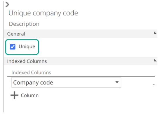 |
The index provides Data Hub with the ability to assert that the Indexed Columns (based on the relationship mapping columns) are indeed unique, that is, able to uniquely identify rows. This removes the warning, and if there are ever duplicate values on the Indexed Columns, model processing will fail. As before, this is the desired outcome. It is worth noting that if there were duplicates on the relationship mapping columns, Model processing would have still failed without this index. However, the index allows Data Hub to identify the root cause of the issue. Where there are multiple lookups on a pipe, this can be a significant time-saver. We have moved quickly through this example because it is covered in detail in the Resolve model common validation warnings How-to article for reference as you need it.
Manual data validation
At this point, you have resolved all warnings, and your model is successfully processing. Or lucky you, your source system was not heavily customized, so the Solution Model worked out-of-the-box. Either way, it is still essential that you manually validate your data.
As introduced previously, manual data validation is performed by comparing reports against the warehouse to source reports. The point of this step is to verify your assumptions about the source. For this reason, the source reports must be generated by the source system or from an independent known source of truth (for example a legacy reporting platform).
This step should be performed for each transaction, and each snapshot Pipeline (recall transaction Pipelines capture movements and snapshot Pipelines capture state). Typical reports are trial balance and inventory reports. The Data Sources and Solutions how-tos provide general guidance on which reports are required, in addition to specific guidance for many supported source systems.
Before moving on, it is worth noting that while performance optimization was introduced before data validation, you should initially only optimize to the extent that it accelerates you towards data validation. Apply the three big-hitters as you model, then move to validation as quickly as possible. Only once your data is validated should you consider the additional guidance from the Modeling Performance Guide. Quite simply, it doesn’t matter how fast it is if it’s wrong.
Adding Data Sources
At this point, you have modeled, optimized, and validated your data. Let’s now look at how you would add additional data sources to your model.
Adding a Data Source
The Data Sources section from the Model tab provides the list of all Data Sources in your model. You can add additional Data Sources with the + Data Source button, as in the following image.
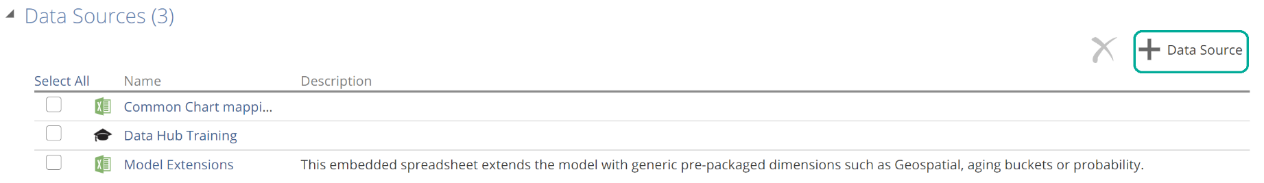 |
You will be presented with a subset of steps from the Model creation wizard, which is where we started this whole journey. The following image shows the Select Source step.
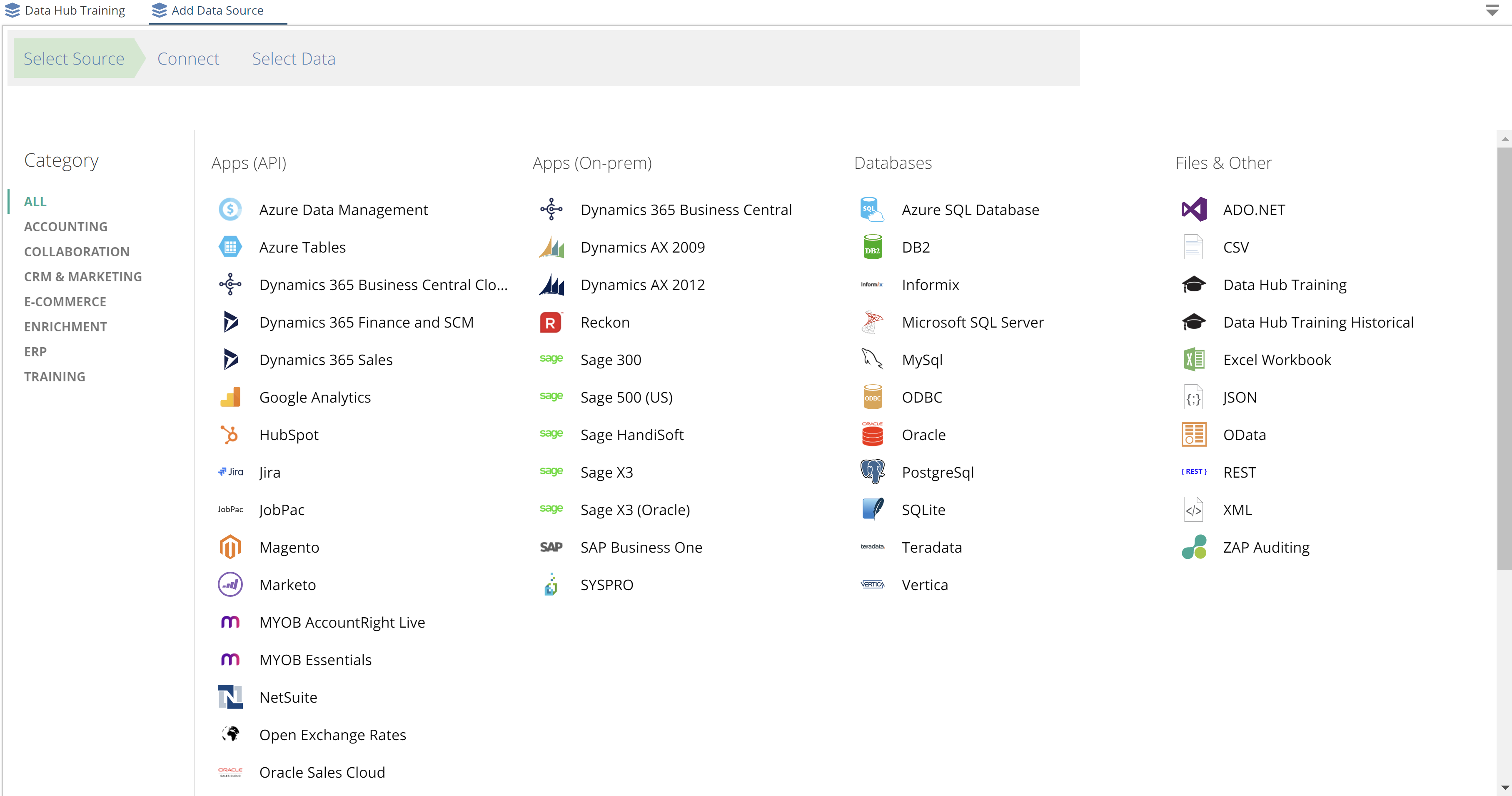 |
Having selected your source, you will see the now-familiar Connect and Select Data steps. Recall Select Data is where you choose the individual Pipelines for inclusion. The Data Hub Modeling Tutorial will provide you with the opportunity to practice adding an additional Data Source to a Model.
Adding a child Data Source
Data Hub provides the ability to merge source collections of tables (schemas) automatically. This is achieved with “child” Data Sources. Child Data Sources are added by clicking + Child Data Source on the CHILD SOURCES tab of an existing (parent) Data Source, as in the following image.
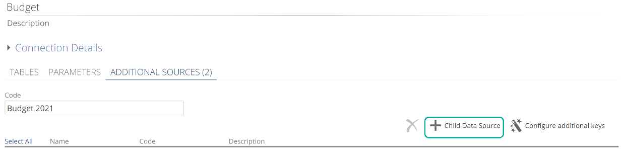 |
Rows for child Pipelines are automatically unioned with rows of the matching parent Pipelines. In this way, complete schemas are merged. It is helpful to compare Schema Merge to Table Merge to aid in understanding both features. Recall that Table Merge is configured with either the Add Pipeline as Union of Tables button or the Tables field from the SOURCE tab. Schema Merge differs from Table Merge as follows:
Automatic table matching – Schema Merge automatically determines which tables to combine into a single Pipeline by matching table names. Table Merge, on the other hand, requires the tables to be manually specified.
Cross-Data Source – Schema Merge works across Data Sources. Table Merge, on the other hand, combines tables within a Data Source.
Tables from a child source that cannot be matched to a parent’s table can be individually added as Pipelines. Sensibly such Pipelines are sourced solely from the child source. From the image above, you may have noted the Configure Additional Keys button. If the merged tables may result in duplicate rows, then you can use this option to include an additional key column. The included key column is based on the Code field specified for parent and each child Data Source, as in the following image.
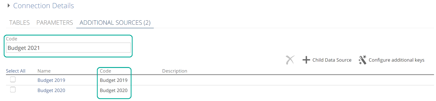 |
One common requirement for child Data Sources is when the source system stores each company’s data in a different database. By choosing the primary company’s Data Source to be the parent, and then adding a child Data Source for each remaining company, it is possible to transparently combine company data to provide a single set of merged Pipelines. If you are connecting to a source known to store information in this way, Data Hub will automatically configure this tab for you.
In another requirement, multiple Excel files exist, all with the same set of sheets, and you wish to combine each set of matching sheets into a Pipeline. For example, each Excel file might have a sheet per region. For this, you will need to configure the CHILD SOURCES tab manually. While the configuration of this tab is beyond the scope of this document, it is a relatively simple exercise given the material we have now covered. The important thing to keep in mind is that these capabilities are available to save you significant time, should you require them. And when you do, use the in-application hover-over tooltips and How-to guide as needed.
Reporting and analytics
Pre-build Analytics
By now, you have all the knowledge necessary to build a complete data model in Data Hub. All we have left to discuss is configuring your model for reporting, and optionally deploying the pre-built suite of analytics for your analytic tool of choice.
Data Hub produces an open-standard SQL database. You can connect to this database from a variety of tools, including Excel and other reporting and analytic tools. And as discussed, Data Hub also provides a suite of pre-built analytics for many Solutions (recall that a Solution is simply a pre-built Model for a specific source). The list of Solutions supported by the pre-built analytics suite is available here. This pre-built suite itself is available for Power BI, Tableau, and Analytics with Data Hub.
The steps for deploying and configuring the analytics can be found in the relevant How-to of the Analytics documentation. For customizing the analytics, please see the relevant tool’s documentation or, in the case of Analytics with Data Hub, it is recommended that you read The Complete Guide to Analytics with Data Hub. What we want to discuss now is how the same suite of analytics may work across multiple Solutions.
Unified Layers
Data Hub delivers the same suite of pre-built analytics across multiple Solutions by standardizing table names, column names, and column data types across Solutions. This is made possible with the Unified Layer resource type. Let’s move straight to an example to make this clear. In the following image, the Unified Layer Step is shown for the Customers Pipeline. If a Unified Layer is applied to a Pipeline, it will appear as the last Step.
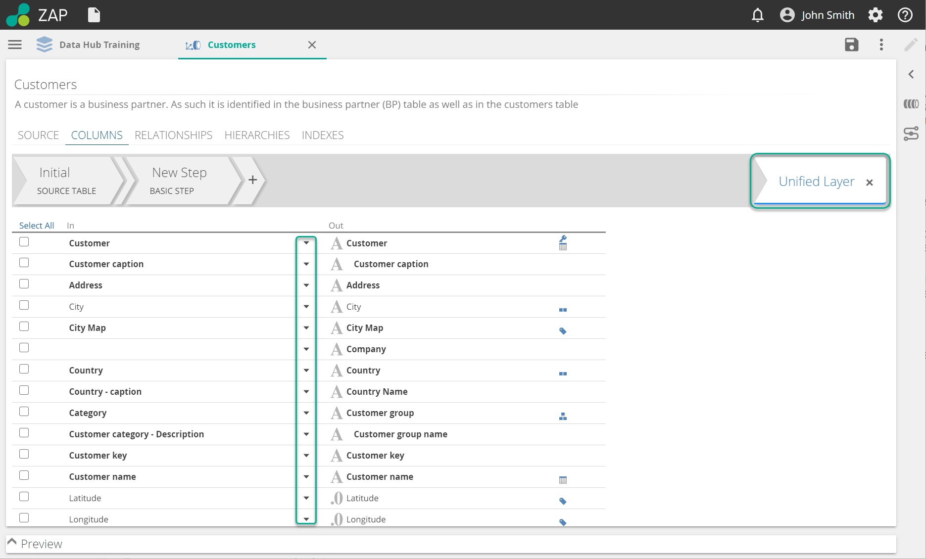 |
The important thing to notice in this image is that many of the rows show a drop-down arrow for the In column. These rows are mapped to the Unified Layer and standardized. For each mapped row, the Unified Layer will override the following properties, and keep in mind your analytic tool may go directly against the warehouse or a semantic layer (if present):
Name – the name of the column in the semantic layer
Data Type – the data type of the column in both the warehouse and the semantic layer
Description – the description of the column in the semantic layer
Physical Name – the name of the column, in the warehouse
We have introduced a concept here in passing here. The physical name of a column, table, or database is the name that is reflected in the warehouse, and it can vary independently of the column, Pipeline, or Model name in Data Hub. This ability to vary independently allows for name changes in Data Hub without breaking reports and analytics against the warehouse (which can continue to use an unchanged physical name). The physical name of an object is synchronized with its Name property by default. The following image shows the configuration options for a column’s physical name.
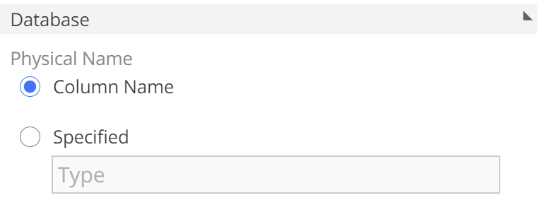 |
Returning to the discussion at hand, in addition to overriding the column properties, the Unified Layer will also override the Pipeline properties, specifically its Name, Description, and Physical Name fields.
So we see that Unified Layers serve to standardize most column and Pipeline properties relevant to reporting. There is one more point to make on standardization. An applied Unified Layer will also serve to standardize the included columns. Observe the warning in the following image.
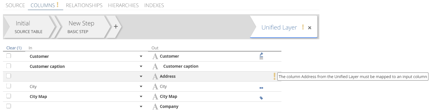 |
This warning only shows for the required column. Not all columns are marked as required on a Unified Layer, but those that do are essential for the operation of the pre-built analytic suite.
Let’s quickly discuss a few properties of Unified Layers:
You cannot perform any transforms on a Unified Layer Step, nor change column names and column types. Given that a Pipeline always opens on the final Step, and this final Step is often a Unified Layer step, you will usually need to select a preceding Step to modify a Pipeline.
You can see which Pipelines have a Unified Layer applied and the name of that Unified Layer from the Pipelines list on the Model tab. Only those Pipelines used directly by the pre-built analytics require a Unified Layer.
Each Pipeline can have a single Unified Layer applied, and each Unified layer can only be applied to a single Pipeline.
You can manually apply a Unified Layer with the steps from the How-to guide. However, if you are using the pre-built analytics, then it is also very likely you are also using a Solution. And in such a case, the Pipeline will already be configured for the relevant Unified Layer.
Finally, given Unified Layers are resources, they are themselves customizable. Keep this in mind, should you find a requirement for standardization across models. However, this customization is beyond the scope of this article.
To sum up, Unified Layers standardize columns and Pipelines across models, primarily for use with a single suite of reports or analytics. In a sense, they provide a contract between the model and analytics. If the model adheres to the contract, then the analytics are guaranteed to work. If you have no intention of ever using the pre-built suite of analytics you may remove the Unified Layer steps so that the final step on each Pipeline is editable.
Security
Once you have a complete Model in place, you may choose to restrict access to this Model’s data. Sensibly the steps to doing so differ significantly based on how the reporting or analytic tool accesses the Model’s data. This access may be against the warehouse or the semantic layer. In both cases, it is possible to restrict at three levels:
Model – Restrict which users may access the Model’s warehouse or semantic layer. Users can be manually granted access rights. Alternatively, it is possible to give rights to all users with access to the Model resource.
Pipeline – Restrict which Pipelines users may access.
Row – Restrict which Pipeline rows users may access.
Whether you connect to the warehouse or the semantic layer, security is configured on the Model Role resource. Details of this configuration are beyond the scope of this article. If you access data from the warehouse, the Secure your model with a Model Role article provides How-to guidance on configuring the Model Role. If you access it instead from the semantic layer, then the Secure your cube article provides the relevant guidance.
Reporting Relationships
To this point, we have used relationships to support lookups. These relationships reside only in the Model resource. It is also possible to define relationships in the warehouse itself. These warehouse relationships may simplify reporting direct against the warehouse. This is because the reporting or analytic tool is already provided with information on how the tables relate. Warehouse relationships are entirely optional. It is also important to understand that warehouse relationships will only result if both the relating and the related Pipeline are configured with Create Pipeline Asset to Table.
To generate a warehouse relationship, check the For reporting check-box in the relationship design panel for the relevant relationship.
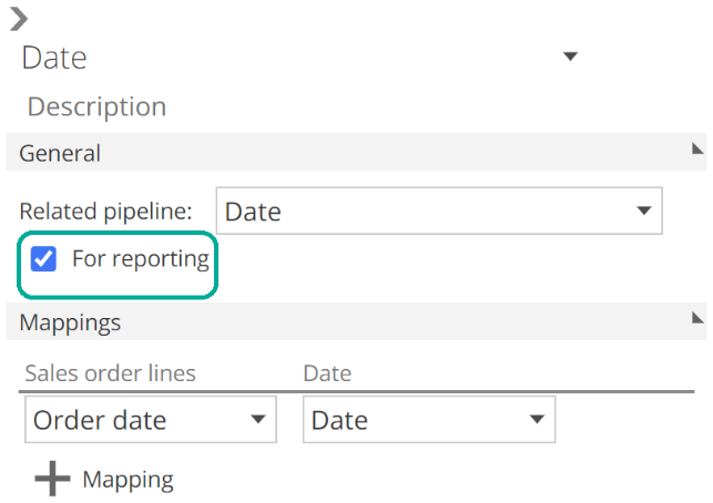 |
A warehouse relationship will also constrain table data to only those rows that can be matched again the related table, or those rows that have empty values for the mapping columns. If any rows violate this matching constraint, then model processing will fail.
You can view all Reporting Relationships for a Model from the Relationships section of the Model tab. This section shows only Reporting Relationships. If you started with a Solution, you would find this list includes many Reporting Relationships preconfigured for your model. The For Reporting check-box also has implications for the semantic layer, which are discussed in the Complete Guide to the Semantic Layer.
Time zone and language
Data Hub provides two model-level configurations for localization, as in the following image.
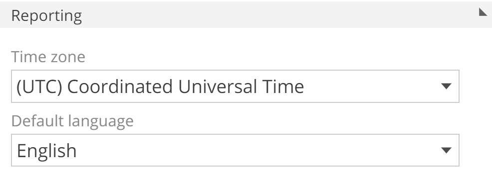 |
The Time zone setting serves two purposes. It affects Process Configuration schedules. And it is also available as a parameter for use in calculations with the Time Zone Conversion modeling function, or in SQL expressions using the #parameter# syntax (see the Parameterize your model to avoid constants article).
Depending on the source system, the Default language setting may be used to pull captions and descriptions for the specific language provided. This field is only relevant when the source includes such captions and descriptions in multiple languages.
The semantic layer
We introduced the optional semantic layer in the modeling architecture section, and we’ve referred to it a few times in passing. The semantic layer is a compelling complement to any warehouse, but there are additional licensing considerations that are beyond the scope of this document. Importantly, Data Hub pre-built analytics are available against both the warehouse and the semantic layer with some caveats as follows:
Warehouse – both Power BI and Tableau analytics suites are available for direct-warehouse reporting.
Semantic layer – Analytics with Data Hub requires a semantic layer. Support for the pre-built Power BI suite against a semantic layer is coming soon.
If your scenario falls under the semantic layer bullet point, we recommend you take some time to fully digest this article, then read the Complete Guide to the Semantic Layer.
Where to next
At this point, you now have a comprehensive knowledge of modeling in Data Hub. Keep in mind the in-application hover-over tooltips as you work with the application. Where you need additional task-oriented guidance, jump into the relevant How-to articles. And for the nitty-gritty, you may refer to the reference articles. From here, we advise the following steps to ensure the success of your data projects:
Familiarise yourself with the documentation for your core Solution or Data Source. The Data Sources and Solutions documentation includes both How-to and reference material.
If you intend to build a model from scratch, it is recommended that you familiarize yourself with the star schema modeling approach. The Power BI documentation provides an excellent article on this topic.
Run through the Data Hub Modeling tutorial (coming soon) or start building out your own sandbox Model as soon as possible.
It is strongly recommended that you challenge yourself against the complete suite of practice problems (COMING SOON).
Keep an eye out for what’s new in the product here.
And finally, this is not intended as a read-once article. We strongly recommend you come back and skim this article after you have a few weeks of data modeling under your belt.
With that… happy modeling!