The complete guide to the Semantic Layer
Estimated reading time: 30 mins.
Welcome
Welcome to this complete guide to the semantic layer. This article intends to provide you with the knowledge required to generate semantic layers for your data models. This article assumes you have previously read The complete guide to modeling in Data Hub. It starts with an overview of star schema modeling before moving on to configuring a semantic model in Data Hub. At the end of this article is a list of next steps that you may consider to bed in the knowledge you gain.
Star schema modeling
The star schema approach
Star schema modeling is the most widely practiced approach to modeling data warehouses and the Data Hub approach. Analytic tools such as Power BI and Qlik are specifically optimized for performance with star schemas. A schema is simply a blueprint for how a warehouse is constructed: how it is divided into tables and how those tables relate. And we will see shortly why this approach is called “star” schema modeling.
Dimension and fact tables
Star schema modeling entails creating separate fact and dimension tables as described below.
Dimension tables describe business entities, for example, customers or sales orders. As another example, Data Hub models create a system Date dimension table by default. The descriptive columns of a dimension table are attribute columns. For example, Day of Month is an attribute column of the default Date dimension table in Data Hub. A dimension table must always provide a key column (or columns) to identify the business entity uniquely.
Fact tables store observations or events, for example, transaction amounts associated with an order. A single fact row can capture multiple observations or events. The observation or event columns are measure columns. In Data Hub, measure columns store numeric values only. A fact table also contains dimension key columns (“foreign keys” in database terminology) for relating the fact table to dimension tables. Because there are generally far more observations or events than business entities, fact tables are usually large relative to dimension tables. Fact tables also tend to grow faster over time.
Note
Both table types can include utility columns that are not otherwise required for the star schema.
Relationships
Now that we’ve introduced the star schema tables recall that a schema also provides how those tables relate: the relationships. Each observation or event row in a fact table relates to a single dimension table row per dimension table, using the dimension key columns. Given most fact tables relate to multiple dimension tables, the diagram of these relationships represents a star, as in the following. Sensibly this is where we get the name for star schema modeling.
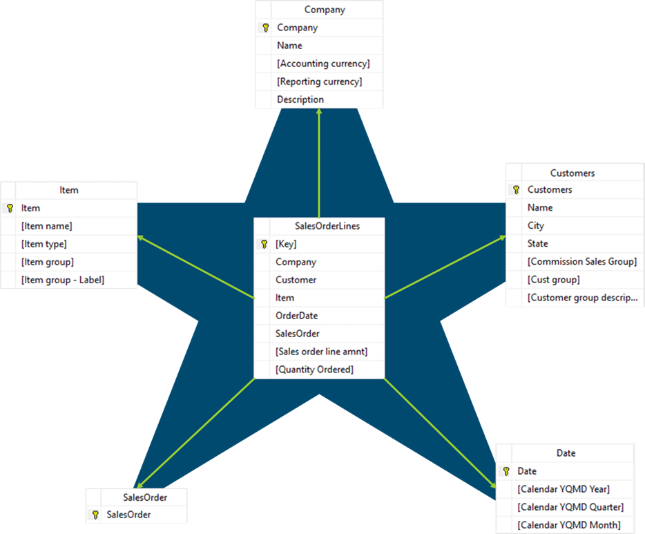 |
Putting it all together
With the relationships in place, it is now possible to use the dimension tables to filter and group the observations and events in the fact tables. And it is possible to summarize these observations and events. That is:
Dimension tables support filtering and grouping.
Fact tables support summarization.
Combination fact and dimension tables
Sensibly, it does not make sense to separate the measure columns and attribute columns into different tables in some scenarios. An example of this is a sales order line table that provides amounts and quantities. It might be necessary to include the order number as an attribute column in the same table to allow for filtering and grouping by order number. In such a case, the table can be treated as both a fact and a dimension table (a “fact dimension” or “degenerate dimension” table for those familiar with the term). Such tables tend to be large and may grow considerably over time. For this reason, this design should be used judiciously.
Modeling for a star schema
Now that we’re familiar with the star schema's basic concepts, we can quickly consider at a high level what the modeling for a star schema would entail in Data Hub. The steps are as follows:
Identify the required dimension and fact tables based on business requirements.
Model the source tables to produce the dimension and fact tables. This modeling predominately entails using look-up columns to construct the dimension tables.
Create relevant relationships from fact tables to dimension tables.
You should already be familiar with look-up columns and analytic relationships from the Modeling Intermediate course.
Note
This guidance assumes relatively modest extensions to an existing model. If you are creating a substantial new model or making substantial extensions to an existing model, please see the Data Hub Agile Methodology to ensure your project’s success.
The snowflake schemas approach
Now for one final schema concept, in particular for the technical audience. An alternate approach to star schema modeling is snowflake schema modeling, where-in the dimension tables are deconstructed (normalized) into component tables. Generally, the star schema benefits outweigh those of a snowflake schema. For this reason, this course will address star schema modeling only, and advanced users are advised to seek additional material if they are interested in this alternate approach. An excellent starting point can be found here. Data Hub fully supports snowflake schemas for the warehouse. Analytics with Data Hub requires a star schema.
Basic semantic modeling
The semantic layer
Now that we have modeled our warehouse, we can discuss the two options available for creating analytics against the data. The first approach is to query the data warehouse directly using Excel, Power BI, or other such tools. Data Hub offers a suite of pre-built analytics against the warehouse, representing a lightweight solution to some analytic requirements.
However, this approach to analytics means that every Excel report or Power BI model must redefine the relationships, summarization, hierarchies, and calculations for each report or model. Each time, the meaning or semantics of the warehouse must be redefined. The solution to this is to capture those semantics once for all reporting and analytic tools to use. This is the purpose of a semantic layer, or simply the layer that defines your data's meaning.
Configuring the semantic layer of a Data Hub model is referred to as semantic modeling, and it primarily involves:
Marking the dimension and fact tables and attribute and measure columns as such.
Marking relevant relationships for inclusion in the semantic layer(Semantic relationships).
We will look at the details of semantic modeling shortly, but first, it is important to know that Data Hub can automatically generate and synchronize two different flavors of semantic layer:
Dimensional semantic layer (cube) – for use by analytics with Data Hub
Tabular semantic layer – for use by Power BI
While these two types' configuration is similar, this course's remainder covers modeling for a dimensional semantic layer for use by Analytics with Data Hub. If you are using Power BI, continue to the Tabular Semantic Modeling course’s Semantic modeling section.
Note
The same pre-built analytics available against the warehouse is also available for the Dimensional semantic layer. Although not available as yet for the Tabular semantic layer, this will become available in future releases.
Dimensions
As we have seen, semantic modeling in Data Hub is primarily an exercise of marking the pipelines, columns, and relationships you previously modeled into a star schema. Let’s first discuss marking dimension tables and attribute columns. A pipeline that generates a dimension table should be marked as a dimension.
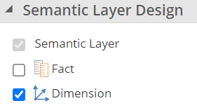 |
We refer to a pipeline marked as such as a dimension pipeline. Each dimension pipeline in a model will generate a dimension in the dimensional semantic layer (commonly “cube”), which reflects on the Dimension Tree in Data Hub as in the image.
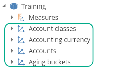 |
Each attribute column and each key column on the dimension pipeline should be marked as an attribute. We’ll talk about the key column requirement later.
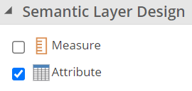 |
Each attribute column will generate an attribute in the semantic layer, reflecting on the Dimension Tree as in the image.
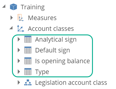 |
Note
We’ll discuss hierarchies (the bottom icon) shortly.
Facts
A pipeline that generates a fact table should be marked as a Fact. We’ll refer to a pipeline marked as such as a fact pipeline.
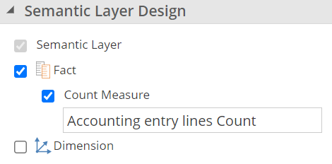 |
Note
You can also include a count column for the fact. This is the single exception where a measure is not sourced from a measure column on the fact pipeline.
Each fact pipeline in a model will result in a Fact in the semantic layer, reflecting on the Dimension Tree as in the image.
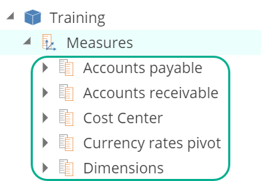 |
As provided earlier, a table can serve as the source of both a dimension and a measure group by checking both Dimension and Fact on the pipeline.
Moving on, each measure column on the fact pipeline should be marked as a measure, and an appropriate Aggregation and Format String should be specified.
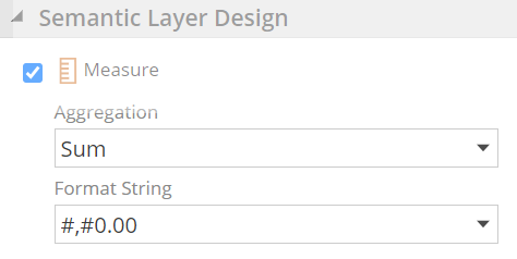 |
Each measure column in a model will measure the semantic layer, reflecting on the Dimension Tree as in the image.
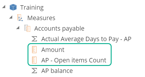 |
Note
Calculated Measures (Actual Average Days to Pay – AP and AP balance), as in this image, are useful at reporting time and are covered in Analytics Intermediate.
Relationships
At this point, we have identified all tables from our star schema that are intended for inclusion in the semantic layer. We did this by marking the pipelines that generate these tables in the warehouse. Keep in mind there are many utility tables and columns that are only intended for the warehouse. Sensibly the final step is to mark the relationships of the star schema for inclusion in the semantic layer.
Relationships intended for the semantic layer should be marked as Semantic relationships.
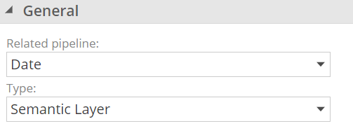 |
Relationships intended only for look-ups should be marked as Lookup relationships to avoid unnecessary or even incorrect relationships in the semantic layer.
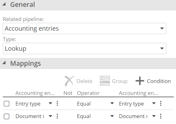 |
Extending a semantic model
At this point, we’ve defined a complete semantic layer, and it’s ready for reporting. However, to satisfy all your analytic requirements, it’s likely that your model will require a little more configuration. We’ll cover this in the following sections.
Dimension keys
As we’ve seen, a dimension table must always provide a key column (or columns), and recall that tables and columns are only included in the semantic layer when appropriately marked. We also covered that each key column on a dimension pipeline must be marked as an attribute.
We didn’t cover that the key columns of a dimension can differ from those of the dimension table. For example, your dimension table may require both a Company and an Account code column to identify an account uniquely. However, if you only need filtering and grouping at the account summarization level (technically, this is the “granularity”), you would only mark Account code as an attribute. The columns list would then appear as follows.
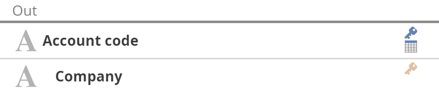 |
Note
The primary key (in blue) selection has implications for reporting and should be the most granular (highest count/cardinality) of the key columns. The key columns in yellow are referred to as “additional key columns.”
Another possibility is that you may not want any of the warehouse’s key columns to be included as attributes in the dimension. Without key columns, other measure groups will not relate to this dimension, so this only makes sense if the dimension pipeline in question is also serving as a fact pipeline. To configure a dimension pipeline without key columns, you must explicitly specify that it is a stand-alone dimension in that it stands alone from other fact pipelines. If this is a little too technical at this stage, be assured in-application validation will guide you when required, and you may refer back here at that time.
Hierarchies
Until now, on to a slightly simpler subject, we’ve configured relationships between measure groups and dimensions. It is also possible to define relationships between attributes to create hierarchies. Hierarchies are an important component for conveying meaning in the semantic layer, and they allow for navigation, particularly drilling up and down.
Hierarchies are configured on the pipeline from the HIERARCHIES tab.
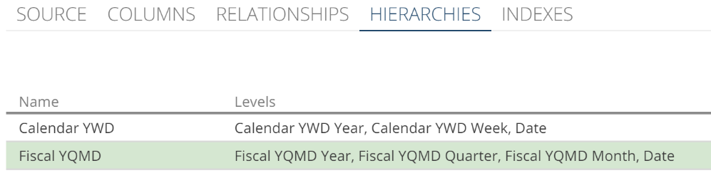 |
A hierarchy is defined by specifying the attribute columns a user would naturally traverse in the processing of drilling down through the data, as in the following image.
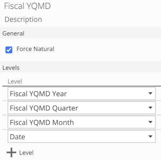 |
Hierarchies can be seen on the Dimension Tree by expanding the relevant dimension node as in the image.
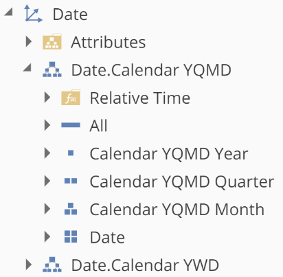 |
Note
For most hierarchies, a value at one level naturally implies the higher level’s value. For example, the 1st July date value naturally implies a July month value. You can optimize such natural hierarchies by checking Force Natural.
It is also possible to configure a parent-child hierarchy where a dimension’s column(s) relates to the same dimension’s key column(s). For example, a Projects dimension may include a Parent Project Id column to specify the parent project. See Add a parent-child hierarchy for guidance on creating parent-child hierarchies.
Additional attribute properties
We previously covered marking attribute columns as attributes. Once marked, the column design panel will show additional properties respective to the semantic layer type you are working with.
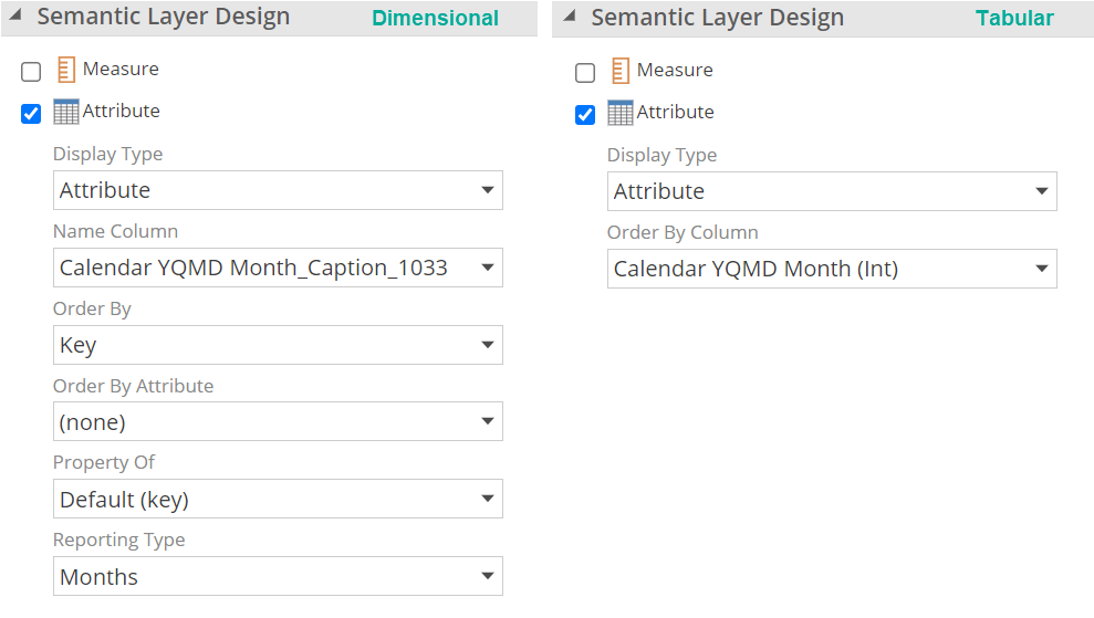 |
We’ll cover these briefly, starting with the Display Type options. The default is Attribute, which includes an attribute column as an attribute in the semantic model. Display Type is the same for dimensional and tabular modeling.
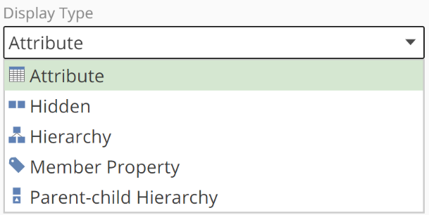 |
The other display types available are:
Hidden – allows for key attributes that not visible in the Dimension Tree, for example, an Id column, and for attributes that are only available as levels in a hierarchy.
Additional columns don’t need to be attributes.
Hierarchy – provides a shortcut to build two-level hierarchies that navigate through the selected attribute column to the attribute column defined as the key.
Member Property – member properties are available in the semantic layer to provide additional information to attributes. You cannot filter or group by a member property. For example, a Product Description column may be included as a member property in a Product dimension. Member Properties are properties of the key attribute by default, and we’ll refer to this shortly.
Parent-child Hierarchy – required for configuring parent-child hierarchies as discussed previously.
The Name Column, Order By, and Order By Attribute settings sensibly control how the attribute is named and ordered on the dimension tree and reports. By default, an attribute’s key and name are the same. That is, a Name Column is not specified.
To specify an Order By Attribute, the required attribute will need to be a property of that attribute using the Property Of field. You can intuitively set the Property Of field for an attribute by completing the sentence, “X is a property of Y.” For example, “Color is a property of Product.”
We previously saw that Member Properties are properties of the key by default. This means they will only be found in the key attribute's Member Properties folder. It is possible to change where a Member Property is available with the Property Of field. Property of columns are indented below the attribute they are a property of in the columns list.
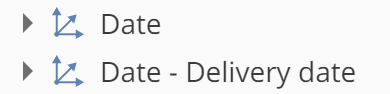
Finally, we have the Reporting Type, which allows you to mark the type for reporting purposes. For example, is it a Date or a City? For Analytics with Data Hub, this setting is only required to customize or create a custom Date pipeline. See the reference article for further information.
In Tabular, there is no concept of a Name column. Instead the columns containing the "display values" are used and becomes the attribute column. In order to specify the same logical ordering, the Order by column property is provided as shown in the image above.
Attribute keys
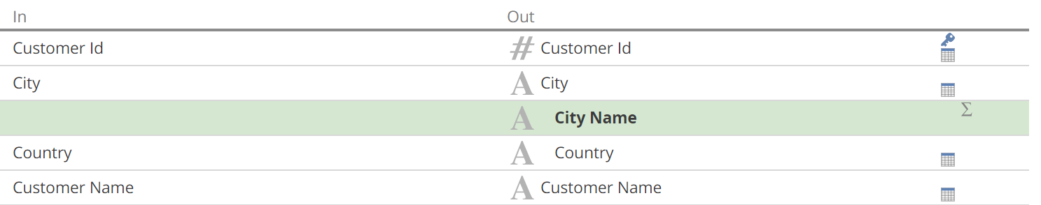
To close our coverage of attributes, we’ll quickly cover the scenario where multiple columns can uniquely define an attribute. To this point, we’ve seen each attribute column is mapped to a single attribute. On occasion, multiple columns may be required, and the Additional key columns field from the report design panel accommodates this. Be aware that this configuration only makes sense with a Name Column that disambiguates the attributes key values, as with the calculated column in the following image:
 |
Resulting in the following preview.
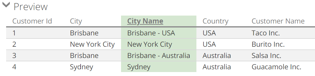 |
Note
The City Name and Country columns are indented below the City column in the previous image. This is because additional key columns and the name columns of an attribute are the key attribute's implicit properties.
Relationships types
There are two additional relationship types to quickly review to close out our discussion of configuring the semantic layer.
A role-playing relationship is a conventional relationship in every sense, except that the relationship’s name differs from the related pipeline’s name, as in the following image.
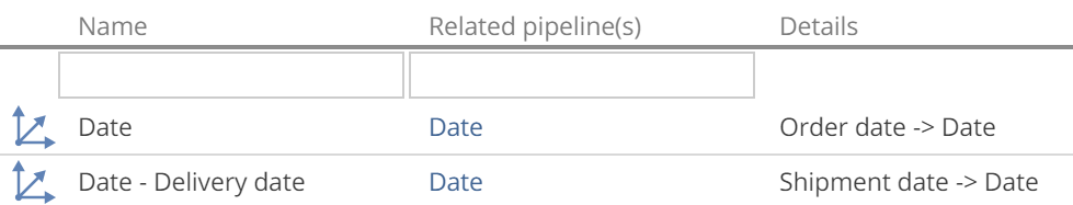 |
A role-playing relationship results in a dimension in the semantic layer named for the relationship name instead of the related pipeline name. The following image shows the resulting dimensions for the previous image's relationships.
 |
Role-playing relationships are useful to allow a fact to be filtered and grouped by the same dimension but based on two different relating columns (order date and shipment date in the above example).
Many-to-many relationships cater to the scenario where an observation or event relates to more than one business entity. The classic example is shared bank accounts, where each transaction must now relate to multiple account owners. Many-to-many relationships can be very powerful. However, they also introduce challenges in building analytics and reports. For the example at hand, merely summing the records for all bank accounts will multiple-count many transactions. See Add a many-to-many (M2M) relationship for how to create a many-to-many relationship.
Model roles and processing
There are two further things to consider with a fully configured semantic layer. Namely, how to secure the data and how to refresh the data.
Data is secured in the semantic layer with Model Roles, as in the following image.
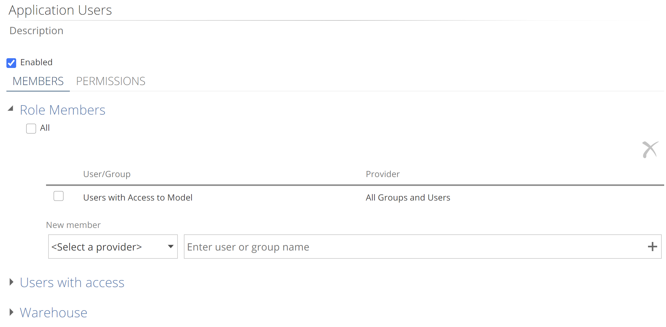 |
The Model Role MEMBERS tab configuration is described in the semantic layer reference article, Model roles. Data permissions are configured on the PERMISSIONS tab. Configuration guidance can be found in How to secure your Semantic Layer.
Data can first be secured by restricting access at the schema level. Once the All checkbox is deselected, you can select whole modules of pipelines for the role.
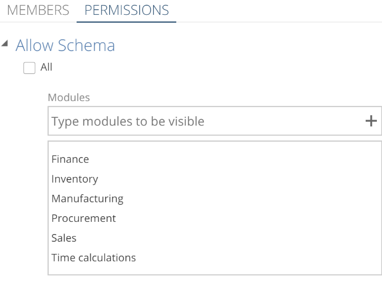 |
See Modularize your Model with Module Tags for configuring the module tags of a pipeline. Rights for individual fact and dimension pipelines can also be granted to the Model Role.
For Dimensional modeling ONLY, one additional level of granular security can be defined with the Limit Data section. This can be done once rights are granted at the schema level. This configuration requires Named Set resources, covered under the Analytics with Data Hub sections of the Data Hub documentation. Once the required Named Sets are created, refer to How to secure your Semantic Layer for the steps to limiting data available to the role.
Publishing and processing
You’re ready to publish! As with publishing the warehouse, publishing the semantic layer updates the structure to reflect your model design, specifically the semantic layer design. And as with warehouse publishing, if you elect to publish and process simultaneously, the publish will not take effect in the event of a failed process. For this reason, it is good practice to publish and process in most cases. This is the default, as shown in the following image.
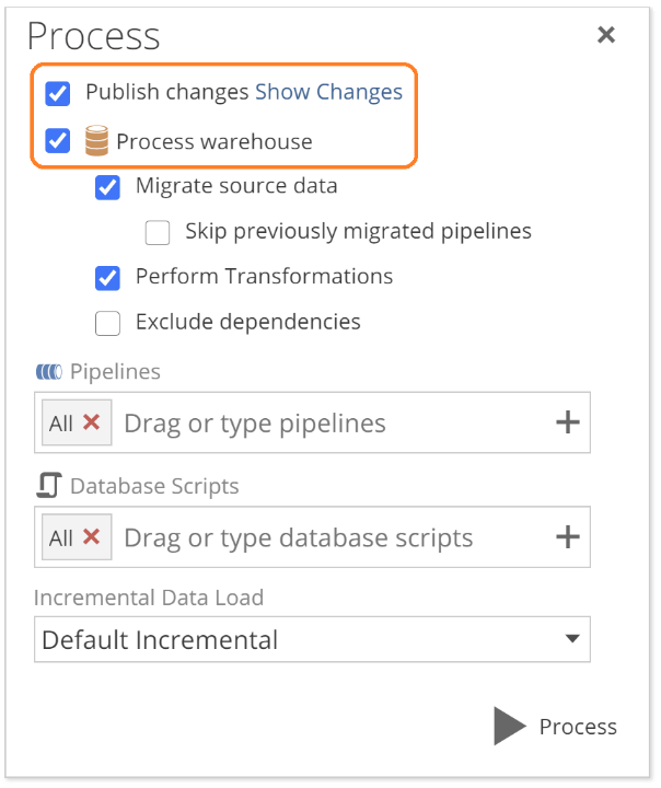 |
While publishing updates the structure, processing updates the data. The semantic layer must be successfully processed to be browseable for reporting and analytics as with the warehouse. That is, an initial Full Refresh must have been performed.
Note
Publishing a semantic layer structure change may require dimension and facts to perform a Full Refresh. Heuristics control when this applies, but it is important to note that a small change may significantly impact processing time.
Warehouse and semantic layer processing are configured together in the pipeline design panel or for the entire model on the data source level. As with the warehouse, incremental load types (data refresh types) are available for the semantic layer.
Dimensional modeling incremental load settings:
Add & Update – rows added or updated are refreshed in the semantic layer.
Add Only – only rows that have been added are refreshed in the semantic layer.
Tabular modeling incremental load settings:
Add Only – only rows that have been added are refreshed in the semantic layer.
Two different Incremental behavior categories are available and can be configured: Default and Quick. These are provided for convenience so that incremental process behavior can be setup per model, or for individual pipelines based on business requirements. Configure on the data source for model level, or if individual settings are required per pipeline, check Override settings from Data Source as seen below.
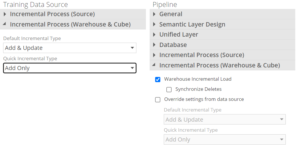 |
The process pop-up is available from either the model design panel or an individual pipeline’s design panel (model design panel shown below).
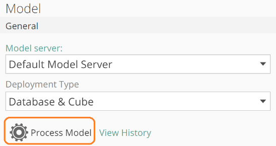 |
The process pop-up and process configuration (see modeling quick start) provide a modifiable field for the list of dimension or fact pipelines to be processed and a dropdown for which incremental behavior should be used across all pipelines.
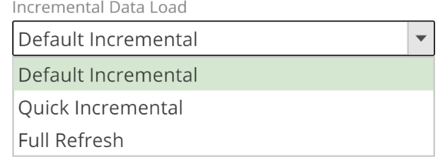 |
The combination of process types and process behaviors allows the designer to specify incremental settings at the pipeline level but still provides a high-level option for Quick Incremental(predominately add-only) processing.
Note
The semantic layer uses the system Zap_CreateTime and Zap_TimeStamp columns to identify added and updated rows. These columns, in turn, rely on correctly configured source incremental settings. Refer back to the Complete Guide to modeling in Data Hub for more detail on configuring source incremental processing.
One additional processing option applies only to semantic models, the Offline option. This takes the Semantic Layer offline while processing, meaning it will be unavailable for reporting until processing is complete. The advantage is that offline processing will use significantly less memory. It can perform the Full Refresh in Offline mode for large cubes in a memory-constrained environment and then perform a Default Incremental refresh online.
Finally, you can see what analytics will be impacted by a data refresh from the pipeline design panel. Expand the Used By Analytics section, as in the following image.
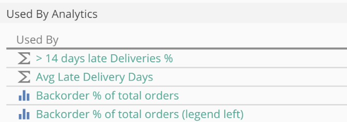 |
Where to next
At this point, you now have a comprehensive knowledge of semantic modeling in Data Hub. Keep in mind the in-application hover-over tooltips as you work with the application. Where you need additional task-oriented guidance, jump into the relevant How-to articles. And for the nitty-gritty, you may refer to the reference articles. From here, we advise the following steps to ensure the success of your data projects:
If you intend to build a model from scratch, it is recommended that you read more on the star schema modeling approach. The Power BI documentation provides an excellent article on this topic.
It is strongly recommended that you challenge yourself against the complete suite of practice problems (COMING SOON).
Keep an eye out for what’s new in the product here.
And finally, this is not intended as a read-once article. We strongly recommend you come back and skim this article after you have a few weeks of semantic modeling under your belt.
With that… happy modeling!