Analytic Functions
By this point, we’ve alluded to Analytics Functions many times. At the same time, you’ve seen all that can be achieved without Analytics Function (or Functions for short). If your data model provides all you need, you may find you don’t make use of Functions for some time. We encountered just such in our very first design example. You may recall we used the Invoice line amounts measure directly on Columns instead of subtracting out the discounts for a Totals Spent column. The model provides a gross amount and a discount amount, but not a net amount (gross – discount). Let’s now demonstrate how we can achieve these Functions.
Value Functions
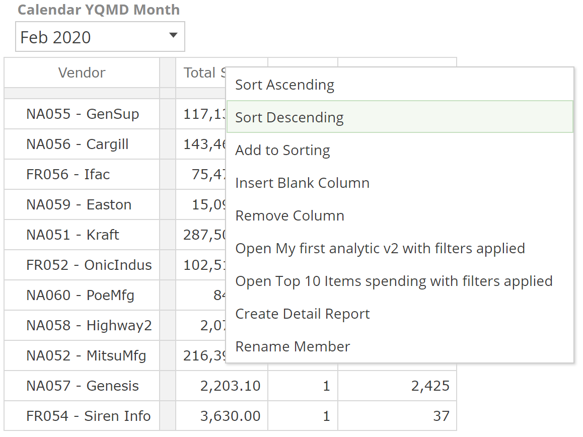
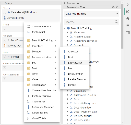
Open and an unmodified version of My first analytic, show the Query design panel, and right-click the Invoice line amounts measure from the Columns placeholder, as in the following image.
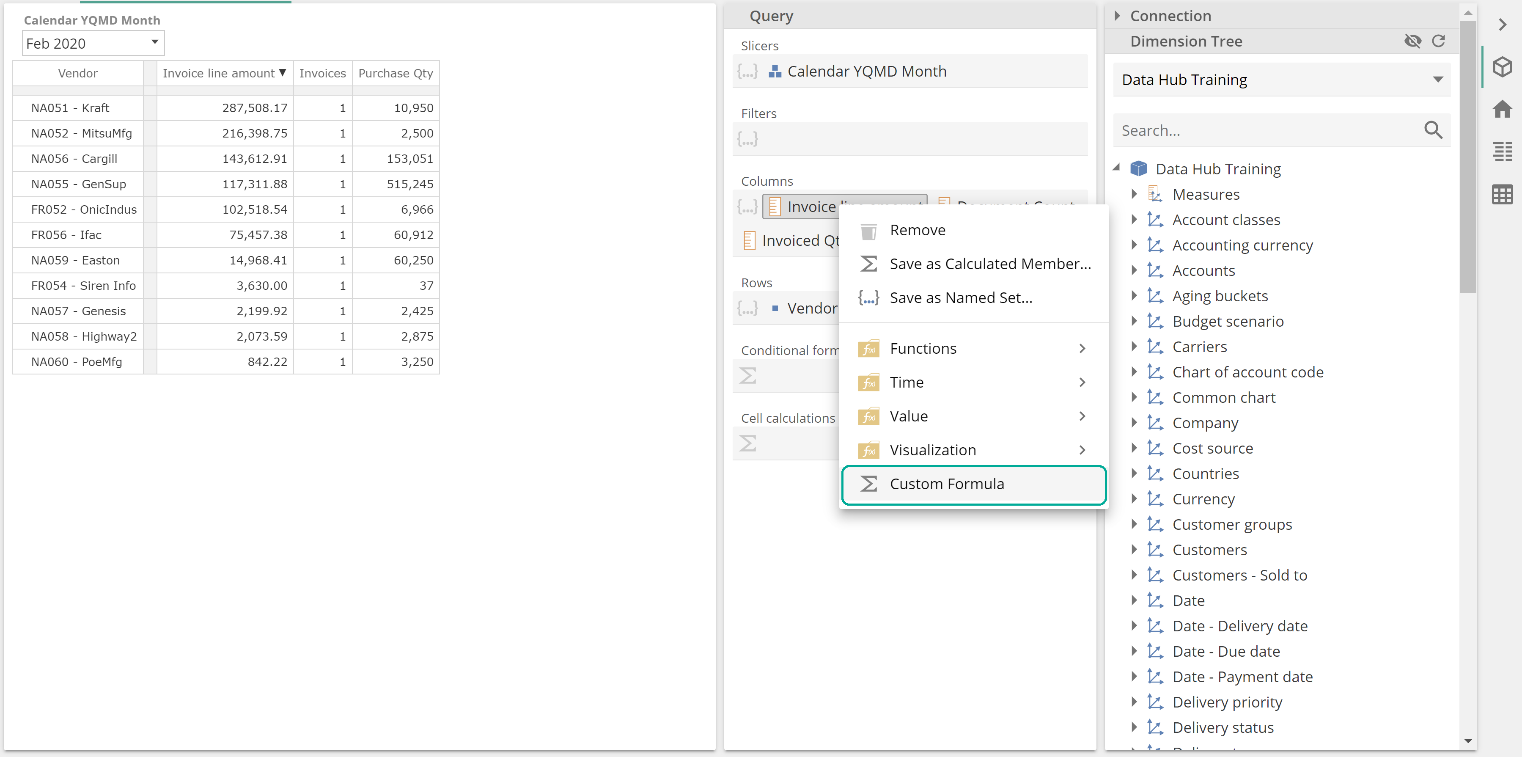 |
We’ll talk about concepts shortly, but we’ll feel this out first. Select Custom Formula from the menu, and the Query design panel will now show as follows.
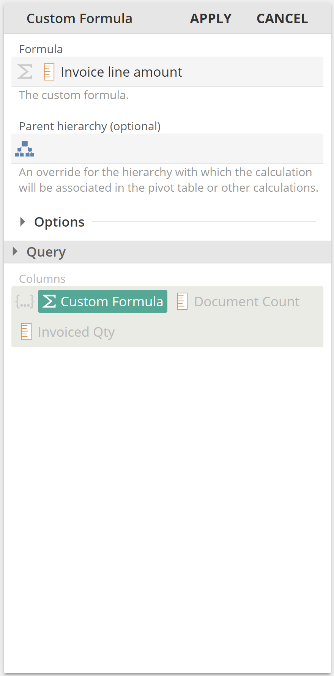 |
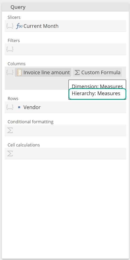
This is quite a change. Where did Rows, Filters, and Slicers go? You can click the Query section header to see them again, as in the following image.
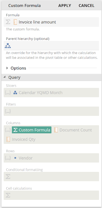 |
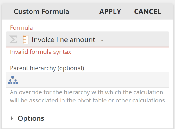
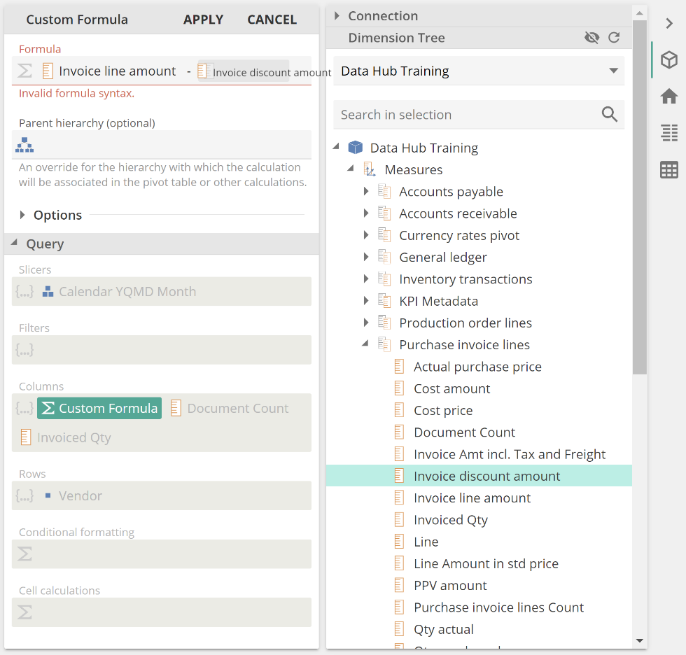
You will note that all of the Query section placeholders are greyed out, and the Custom Formula is highlighted in green. There is also a new Custom Formula section at the top. These changes reflect that we are now defining our Custom Formula, and the Query placeholders are locked until we are complete. Focusing on the Custom Formula section at the top, click in the Formula placeholder and enter the subtract sign, then click Enter.
Sensibly, the formula syntax is invalid at this point, and the application kindly tells us so.
 |
Now left-click and drag the Invoice discount amount from the Dimension Tree's relevant location as in the following image.
 |
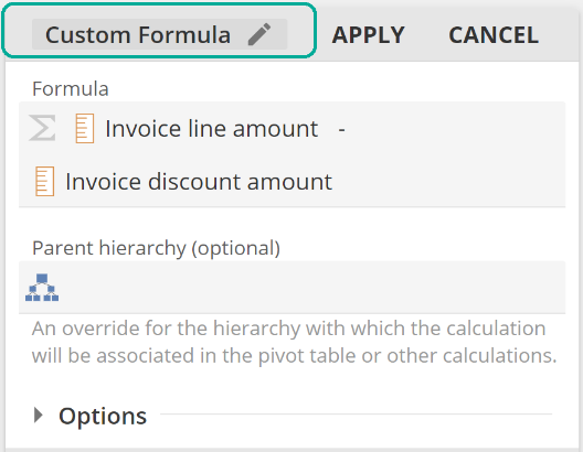
Hover over the Custom Formula section header, and you will see that this text is editable (you will also see a description field in the edit popup).
 |
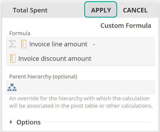
With your formula name specified, click Apply.
 |
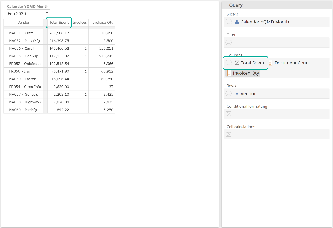
By applying the changes, we have now completed the definition of our new Custom Formula (Total Spent). The table updates to reflect our change, as does the Columns placeholder, as in the following image.
 |
You will notice that our sorting was lost. Because sorting was defined on the Invoice line amount measure, which no longer exists on the table, we must re-apply it (Sort Descending from the right-click header menu).
 |
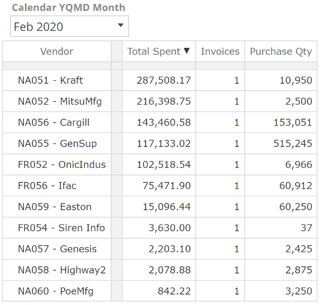
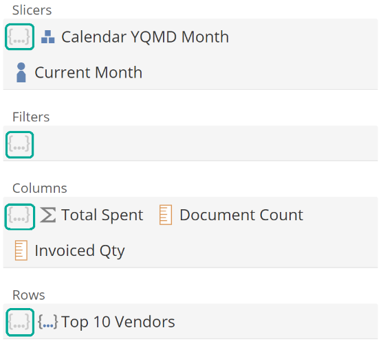
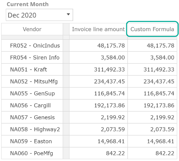
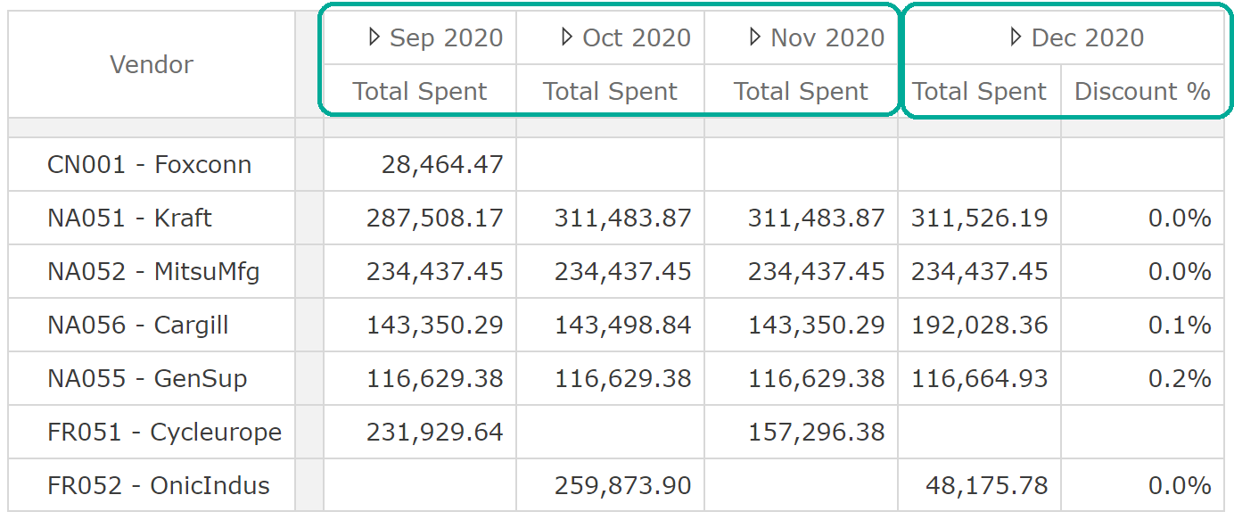
From the following image, you can see we are now a step closer to reproducing the bottom left cell from the pre-built Purchase manager dashboard.
 |
We have just made use of a Value Function. Sensibly Value Functions return values. Again, we’ll go deeper into the concept shortly.
Set Functions
To come closer to reproducing the bottom-left cell from the pre-built Purchase manager dashboard, we now need to change our table's rows only to show the top 10 vendors (for the given Slicer selection). For this, we make use of a Set Function that returns, you guessed it, a set and specifically the set of top 10 members.
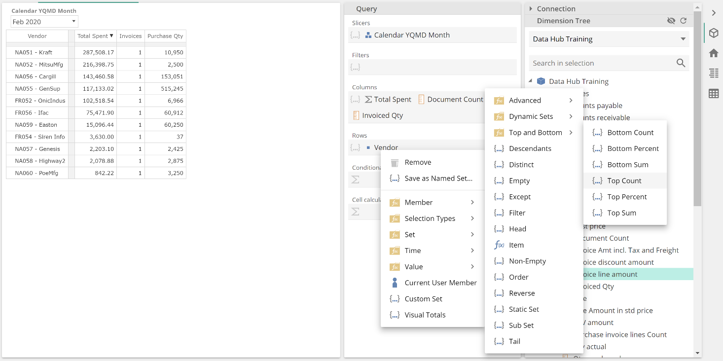
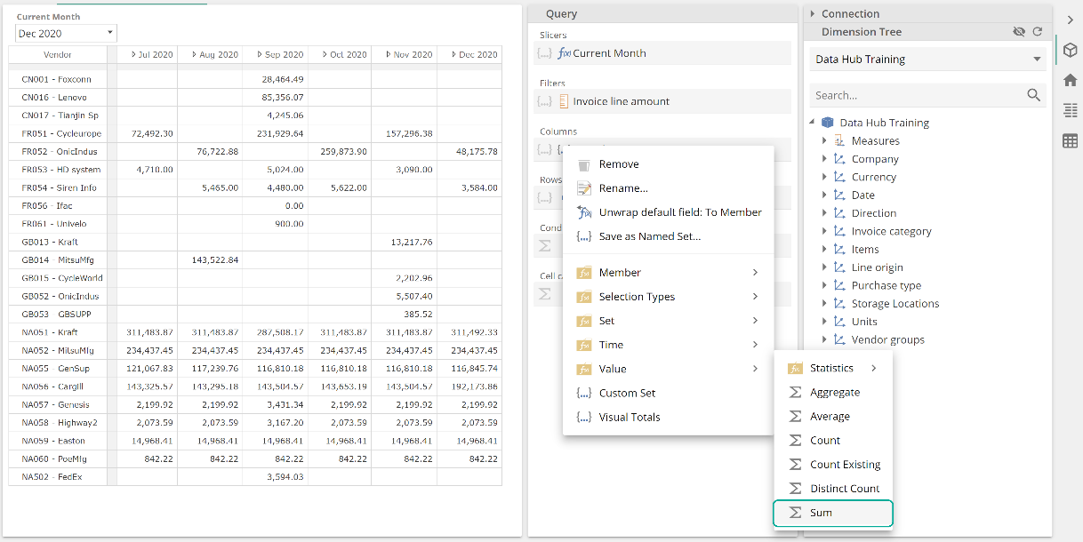
From the Query design panel, right-click on Vendors level from the Rows placeholder and find the Top Count function from the Functions menu (do note its location in the Set folder).
 |
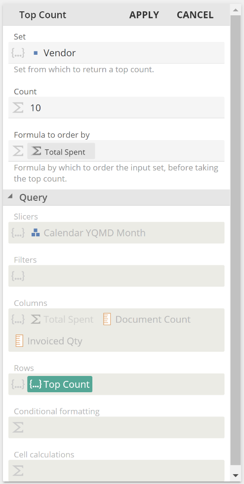
Having selected this Function, the Query design panel will show the following.
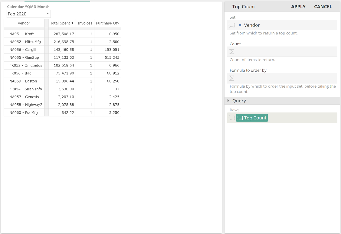 |
Again the Query section is collapsed because we can only work in one context at a time. We are currently working in the Top Count context. Even with the Query section collapsed, we still see Top Count in our Rows placeholder. This helps us track our context; that is, our context is currently the Top Count Function within the Rows placeholder.
Click in the Count placeholder, enter the number “10,” then click the Enter key. We want to order our top count by the Total Spent formula we previously defined. We will need to expand the Query section to see Columns. Drag the Total Spent Formula from Columns to the Formula to order by placeholder as in the following.
 |
Once you release your mouse, you will find the Formula to order by placeholder includes a Reference to Total Spent tab, as in the following image.
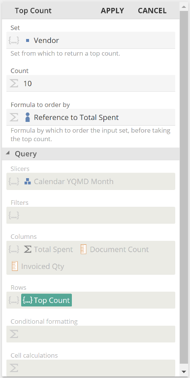 |
We will talk to referencing in a later section, but what’s important here is that should the Total Spent formula change, the Top Count Function must reflect that change. That is, it should be a reference to the Total Spent formula and not a copy.
Because it is the members of a set that show on a table, the set itself's name is not important from a formatting perspective. However, appropriate Function naming (and description) makes for a self-documentation analytic. So let’s quickly update the Function name and click Apply.
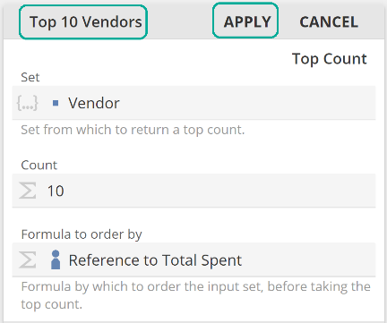 |
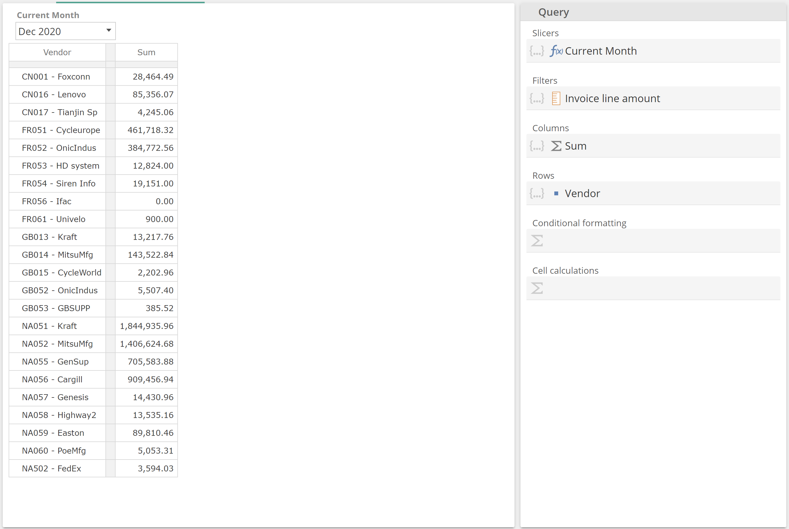
The result is the following.
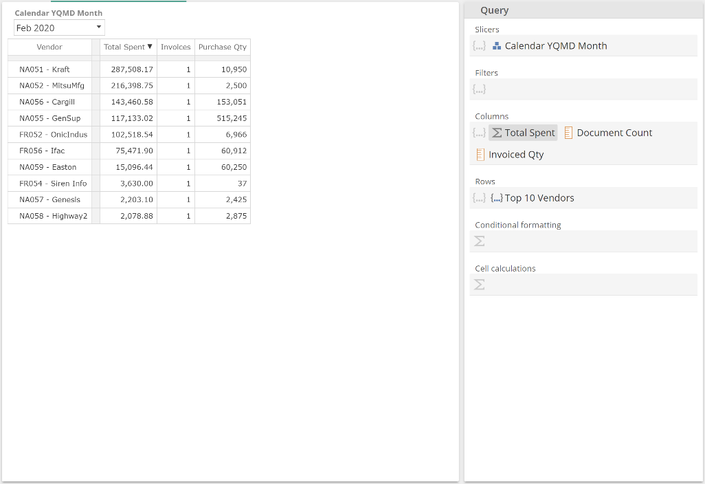 |
Because there weren’t many different vendor sales in the selection month, our Top Count function's effect is a little subtle, but if you look at the table carefully, you will note that there are now exactly ten rows, where previously there were a few more.
Member Functions
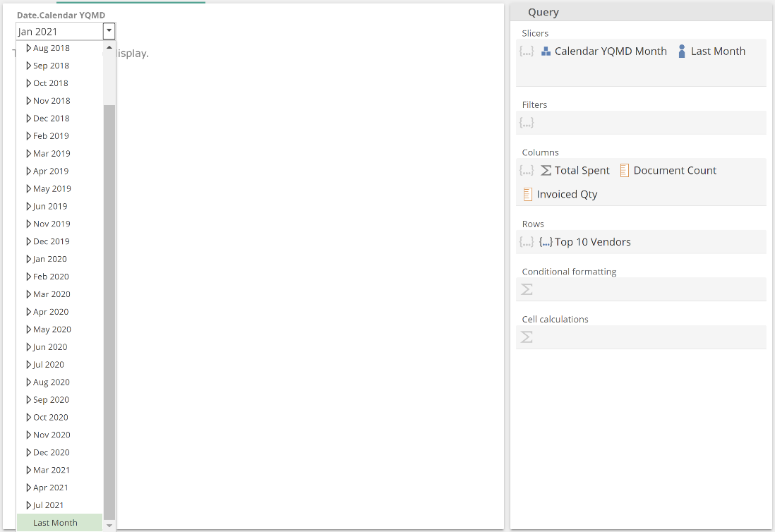
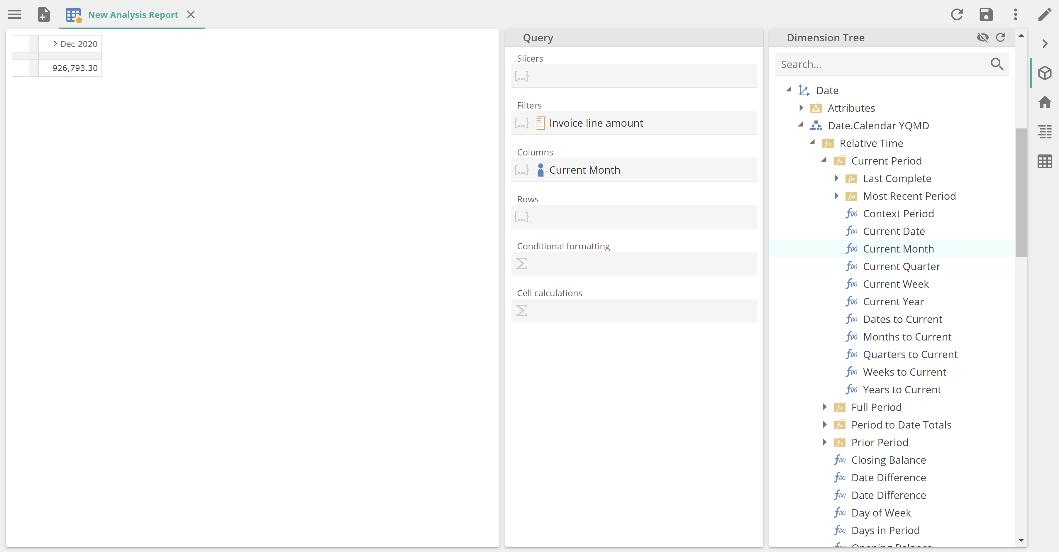
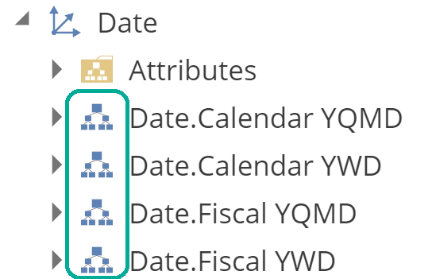
Let’s walk through one more Function type example before we discuss theory. This time, we’ll configure the Function using a different workflow, specifically dragging the Dimension Tree Function. From the Query design panel, expand the Date dimension, the Date.Calendar YQMD hierarchy, the Relative Time and Current Period folders, and hover over the Current Month Function.
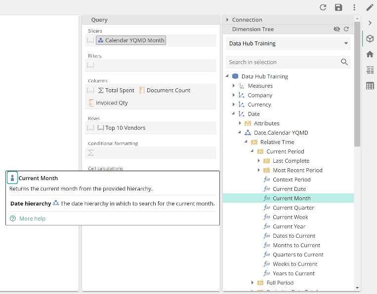 |
Hovering over a function from either a right-click menu or the Dimension tree shows summary information about the Function. An icon to the left of the Function name also indicates the Function type. In this case, we can see a member icon that matches the member icon from the Dimension tree. Sensibly this Function will return the current month member. Drag it to the Slicers placeholder.
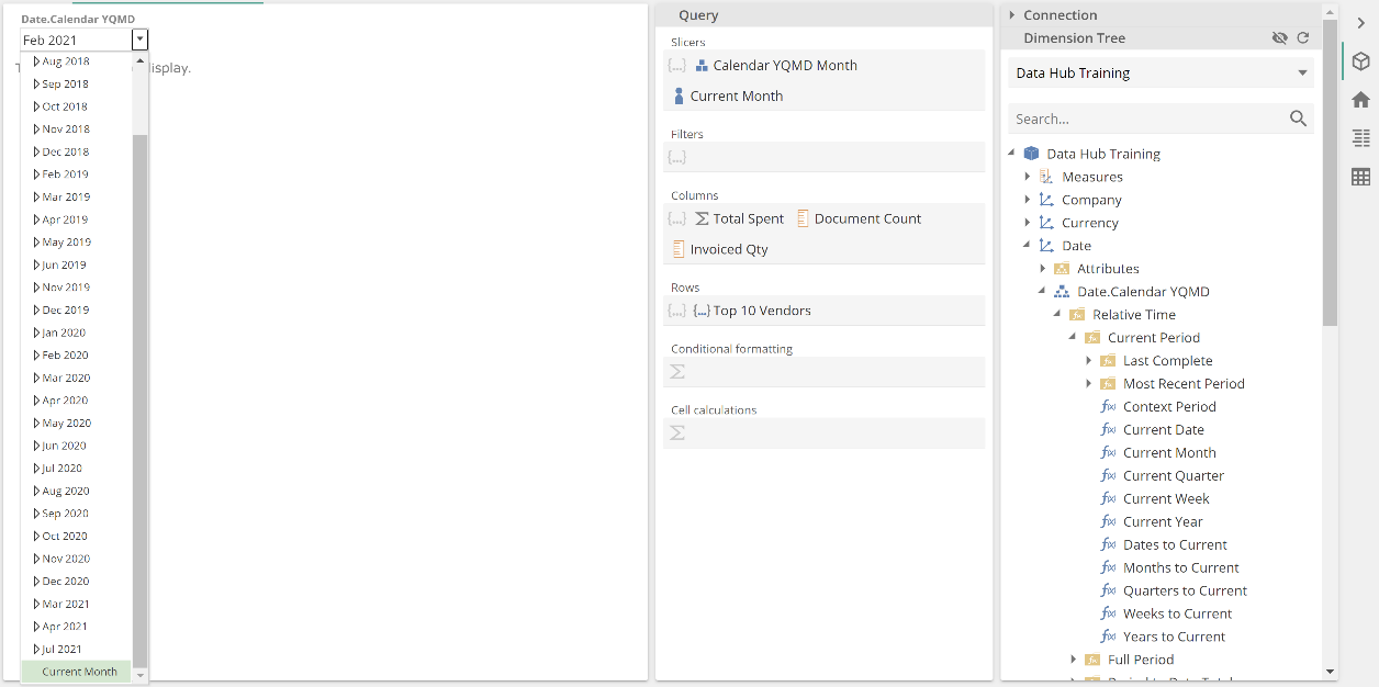 |
This example allows us to demonstrate both a Function that returns a member (a Member Function) and a unique property of Member Functions when used in the Slicers placeholder. From the image above, notice that Current Month is selected from the drop-down; however, Feb 2021 shows in the box. That is, the selection is the dynamic value that the Current Month Function returns, and each time this analytic is opened, the selection will be reevaluated. Again, this is a unique property of Member Functions when they are used in the Slicers placeholder. Please take a minute to save this My first analytic in its new state.
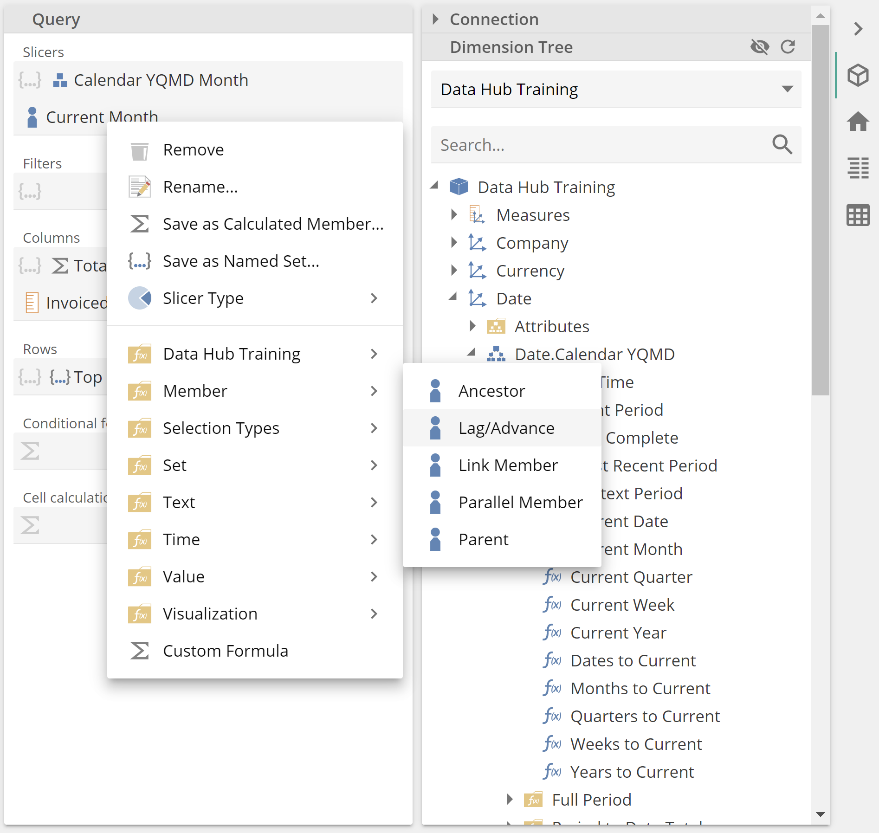
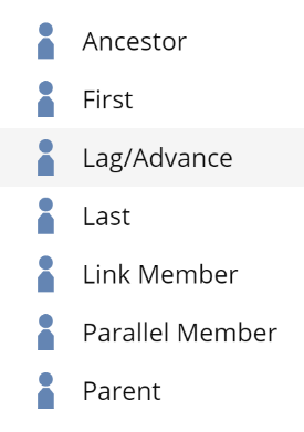
This example was slightly different from previous examples in that our Function didn’t require us to fill any placeholders. We can take this example and build on it to make it a little closer to what we saw with Value and Set Functions. Now right-click on Current Month from the Slicers placeholder and select Lag/Advance from the Functions menu.
 |
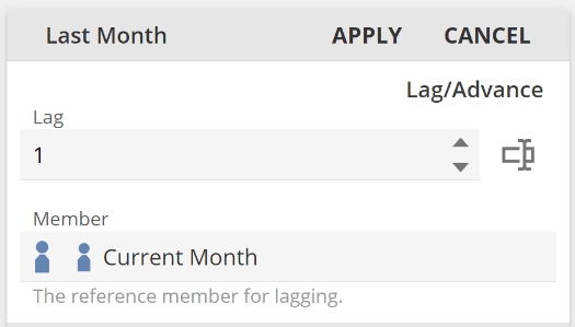
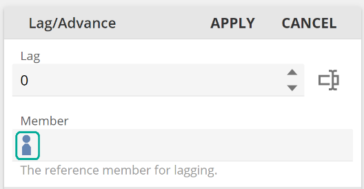
Set the Lag placeholder value to 1. It would also be a good update to rename the Function to Last Month. Click Apply.
 |
If we now select Last Month from the Slicer, notice that the month preceding that from our previous example is now selected.
 |
And again, because Last Month is also a Member Function (it returns a member), the selection is the dynamic value that Last Month returns, and each time this analytic is opened, the selection will be reevaluated.
Function fundamentals
At this point, we are ready to introduce a little theory. So far, we have introduced three different Function types, specifically Value, Member and Set. There is a further fundamental Function type named Logical that returns either true or false. We won’t review a worked example, but below is the Contains Member Logical Function that returns true if the provided member exists within the provided set.
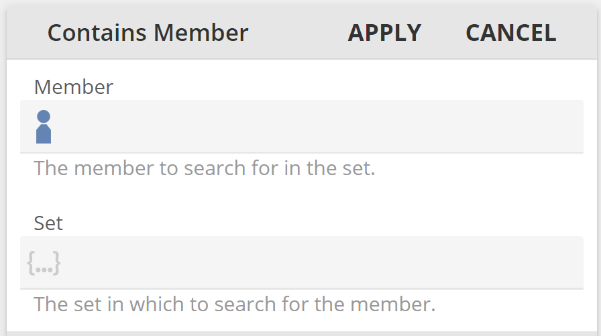 |
All analytics may be built making use of these four fundamental types. As you work to implement a requirement, you should review the Function documentation to find the appropriate Functions from these four types. We will see additional specialized Functions in future sections. These Functions will, however, be specialized versions of the fundamental (for example, a Time Member Function) or special-purpose function (for example, a Conditional Formatting Function).
Placeholder menus
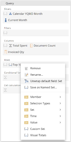
Until this point, we have only seen the Functions menu shown by right-clicking a tab within a placeholder. This is the placeholder tab menu. This menu pre-filters the available options based on the selected tab and the containing placeholder. To best demonstrate this point let’s introduce the second Functions menu that is available by right-clicking the placeholder itself. This is the placeholder menu.
In order to demonstrate this, we’ll continue to work with My first analytics but let’s revert the top-ten change to rows. Don’t save the changes we’re about to make. From the Query design panel, right-click Top 10 vendors and select Unwrap default field: Set.
 |
This action unwraps the contents of the Set field from its outer Top Count function. The result is as follows.
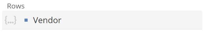 |
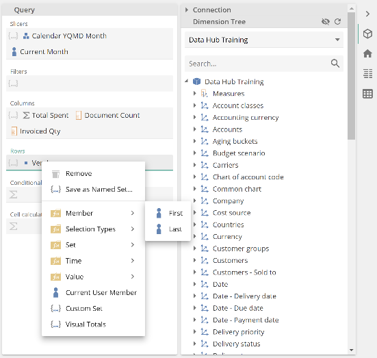
We’ve just introduced the default field in passing. We’ll talk about it more very shortly. Now, right-click the placeholder itself, importantly, to the right of the Vendor tab. This is the placeholder menu. You should be able to find Lag/Advance in the menu, as in the following image.
 |
Don’t select this function. Instead, right-click on the Vendor tab and again search for the Lag/Advance in the menu. This is the placeholder tab menu. You will find Lag/Advance is missing, as in the following image.
 |
Finally, click on Total Spent from the Columns placeholder and right-click in the Formulaplaceholder, importantly, to the right of the measure tabs. Again, this is the placeholder menu. You should see the Logical folder that wasn’t previously available.
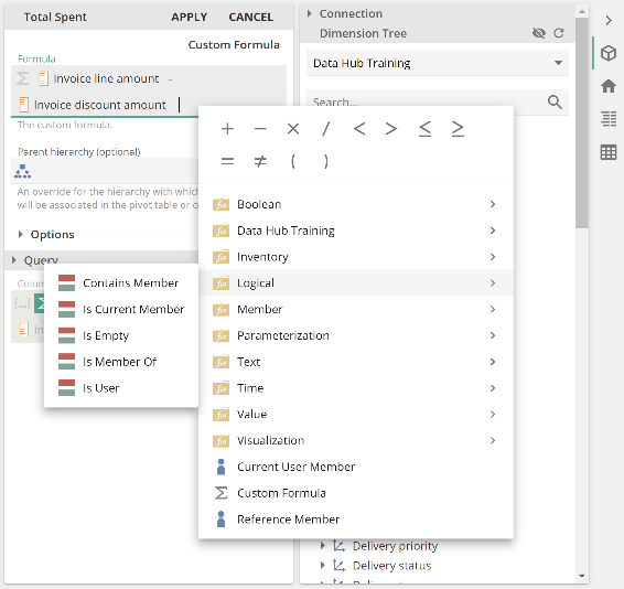 |
To describe this behavior, let’s start with placeholder menu filtering. We saw the placeholder menu twice (and the placeholder tab menu once). We saw it once for the Rows placeholder and then for the Formula placeholder (inside Total Spent). The Formula placeholder menu included the additional Logical folder. Logical functions return true or false values. A set is a set of members and not a set of values. Therefore, the application does not allow you to place a Logical function directly into a set. So we see, the placeholder menu is filtered to only show Functions appropriate for the given placeholder type.
We’ve only discussed Function types until now. The bolded statement above now introduces placeholdertypes. Fortunately, the most common placeholder types are the familiar Value, Set and Member. We’ll talk to additional types in later sections. In the example at hand, Formula is a Value placeholder, and this is identified by Sigma, as in the following image.
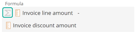 |
The Slicers, Filters, Columns, and Rows placeholders are all Set placeholders, as identified by the set icons.
 |
So we can say, “we didn’t see the Logical folder in the Rows placeholder because it is a Set placeholder, and Set placeholders do not accept Logical Functions directly.”
Let’s now turn to the Lag/Advance Function. We saw that right-clicking in the Rows placeholder showed the Lag/AdvanceFunction. What we’ve not called out until now is that Function types are indicated by an icon to the left of their name in the menu. We can see Lag/Advance is a member Function, as in the following image.
 |
Again, a set is a set of members, so it is perfectly acceptable to show the Lag/AdvanceMember Function in the Rowsplaceholder menu. Why didn’t we see it when in the Top 10 Vendors placeholder tab menu within the Rows placeholder?
To answer this, we need to understand that when we use the placeholder tab menu, we take the current tab, place it in the primary (first) placeholder of the selected Function, and then replace the tab itself with the Function. We call this wrappingthe tab in a Function, and importantly this action populates two placeholders:
The primary placeholder of the selected function is populated with a tab (the Vendors level in our example).
The outer placeholder (Rows in our example) is populated with the Function replacing the tab.
And because we’re now populating two tabs, the application filters the placeholder tab menu to only those Functions that satisfy the requirements of both placeholders.
Armed with this new knowledge, let’s return to the question of why we see Lag/Advance when in the Vendors placeholder tab menu? When we show the placeholder tab menu for the Vendors level, the menu is filtered for those functions that:
Can accept a set (the Vendors level) for the primary field.
Can be placed in a set placeholder (the Rows placeholder).
If we look at the primary placeholder of the Lag/AdvanceFunction, we see it is of Member type.
 |
The application does not allow us to place a set in a Member field, and this is the reason why we don’t see Lag/Advance in the Vendors placeholder tab menu.
We took pains to work through that example because Function-menu-filtering is an important concept to understand. You will need to be able to decide between the placeholder menu and the placeholder tab menu for various actions as you build our more complex analytics.
Working with placeholder types
The previous example also provides a lead-in to another concept. We saw that a Set placeholder (as a set of members) might accept a Member Function. If the Function type matches the destination placeholder type, then sensibly, the Function will show in the menu. There are, however, some additional filtering rules to be aware of. There are as follows:
Value placeholders– accept Value Functions and Logical Functions (in addition to relevant Dimension Tree items)
Member placeholders– accept Member Functions and Value Functions (in addition to relevant Dimension Tree items). A Value Function provides a name for its contained Formula, and that name-and-formula combination allows that it now be treated as a member or measure. A formula without a name is not a member.
Set placeholders– accept Set Functions, Member Functions, and Value Functions(in addition to relevant Dimension Tree items). Value Functions are treated as members, as from the previous point. We saw an example of this behavior when Total Spent (a Value Function) was placed in the Columns (Set) placeholder.
There are a few other such rules that you may encounter in the application. However, menu filtering ensures that you are guided down the correct path in your analytic development. It is strongly recommended that you now take a few minutes to play around with placeholder menus and placeholder types. This will help you build your intuition for working with Functions.
Time Functions
We previously introduced the four fundamental Function Types. Time functions may take the form of any of these four fundamental types. However, they also have either an optional Time Member placeholder or a Date Hierarchy placeholder.
Let’s talk first to Time Member placeholders. “Time” is used here, in the sense that we want to create analytics to reflect data changes across time, whether the time frame is days, months, or years. Time functions do not work on time in the sense of time-of-day. A Time Member placeholder takes any member or member Function from a Date hierarchy because a Date hierarchy describes model data across time. “Date” is used here to reflect that it is a hierarchy of dates.
Again, the Time Member placeholder is optional, and we’ll see why, but let’s first walk through an example in which we populate the placeholder. In so doing, we won’t initially be making use of Time Functions' specialized capabilities, but this approach will allow us to compare and contrast.
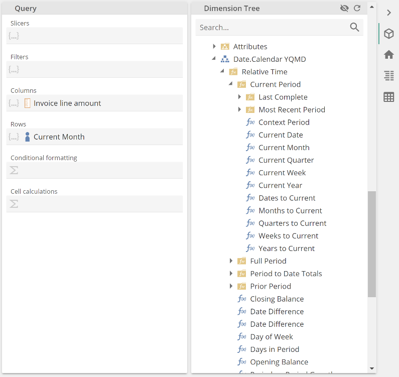
To get started, create a new Analysis Report, place our familiar Invoice line amounts measure in Filters. The drag the Current Month Function from the Date.Calendar YQMD hierarchy's Relative Time folder to the Columns placeholders, as in the following image.
 |
Now right-click the Current Month tab to show the placeholder tab menu and select Year to Date Total (YTD).
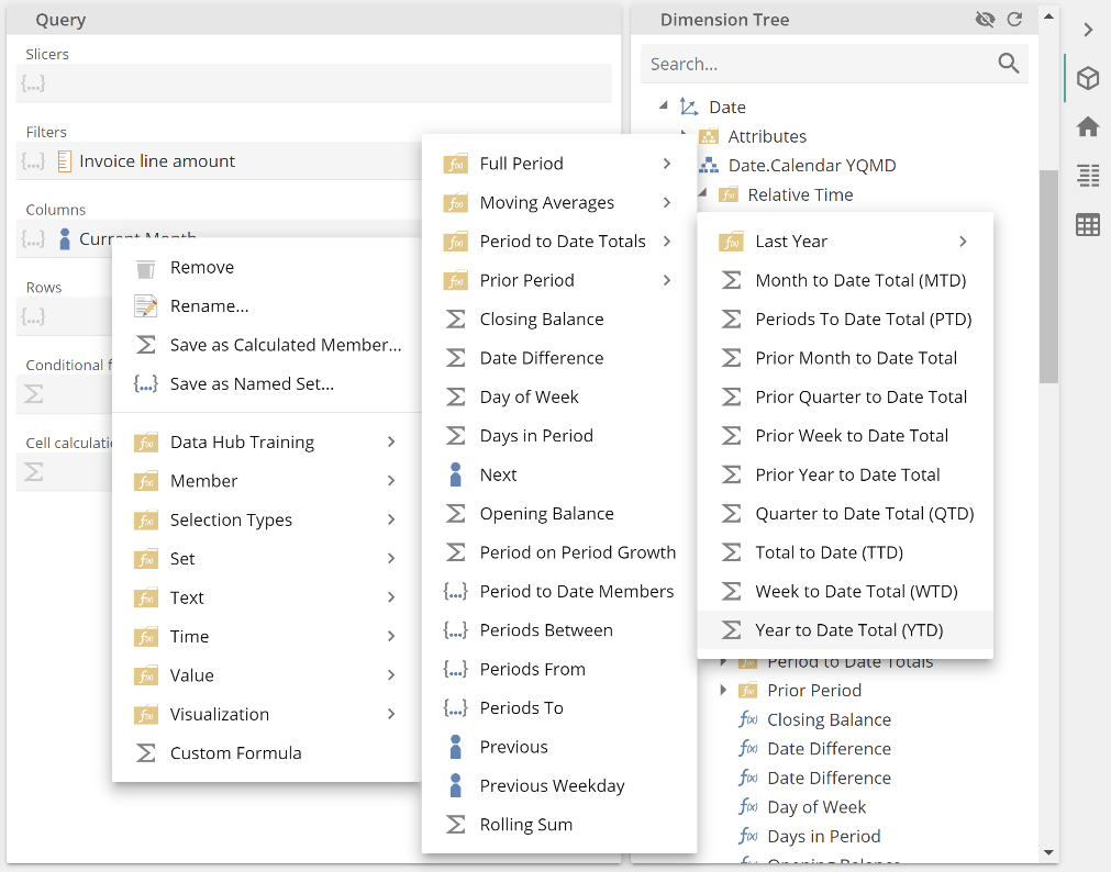 |
As from our previous discussion, this placed the Current Month function in the primary placeholder of the Year to Date Total Function and replace Current Month in the Columns placeholder with Year to Date Total. This can be seen in the following, and note that the Function name defaults to the bracketed acronym where one exists (YTD in this case).
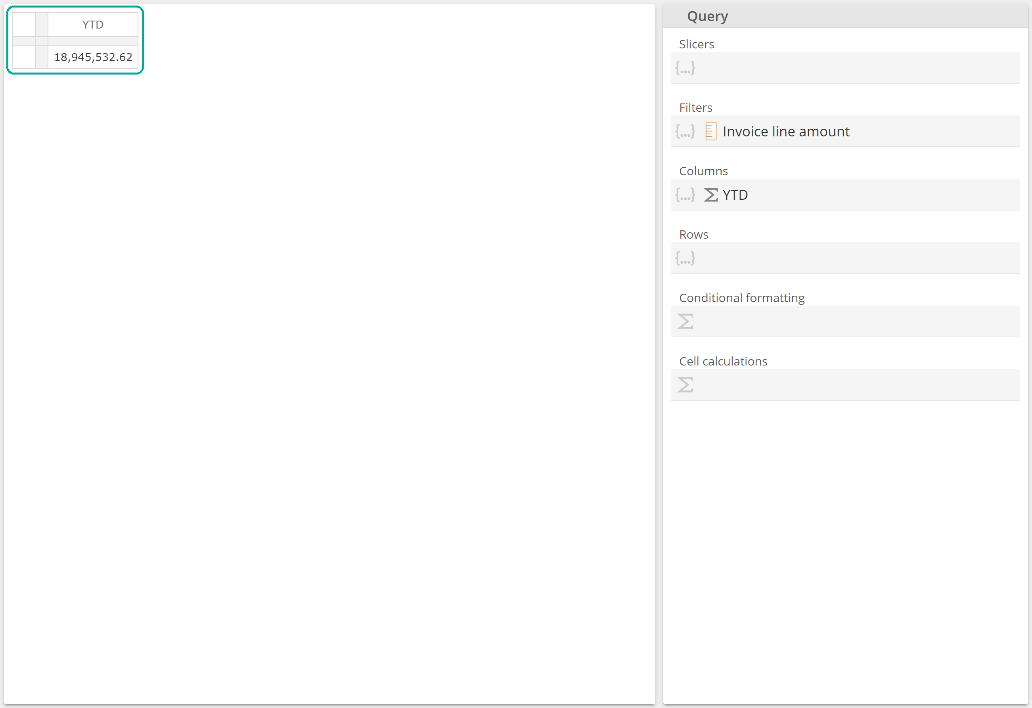 |
The first thing to note is that our table has been updated, and the value is certainly a lot larger than when it showed for the current month alone. It’s also worth noting that this table is not terribly helpful because it’s not evident what month the year-to-date total is for. In many cases, a Slicer is used to provide context to a table, but also, it’s not uncommon to see tables designed to only show current-period data and some period-to-date totals, as in this case. One solution to removing this ambiguity would include “Current Month” in an Analysis Report’s title. But a more time-relevant solution is to make use of dynamic captions. So, before moving on, take a quick foray into the useful feature of Functions.
Click on the YTD function in the Columns placeholder. Firstly, you will note the Current Month function in the Time member placeholder. Time member is not the primary placeholder, but if you wrap a Date-hierarchy member in a Time Function, the Time member is treated as if it were the primary field for that single action. Had we, for example, instead wrapped a measure (which is sensibly a non-Time member) in the YTD function, it would have been placed in the primary Formulate to aggregate placeholder.
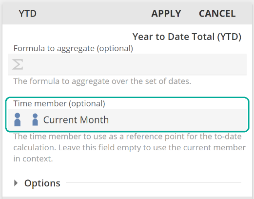 |
Moving on, our goal here is to improve the table. Specifically, we want to change the YTD column header on the table to reflect YTD <current month>. This is configured by expanding the Options section and making use of the Caption placeholder. Drag another copy of the Current Month Function (from the same location as previous) to the Caption placeholder. This now allows us to use the @@ syntax in the function caption field, as in the following image.
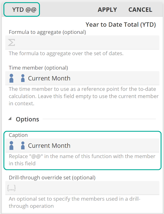 |
Our table now reflects the dynamic caption as a column header. Dynamic captions can also be used with non-Time Functions, but by far the most common scenario is to use them with Time Functions, as was the here.
Let’s now look at the scenario where the Time Member placeholder is not populated. This will introduce us to the unique properties of Time Functions and the significant degree of flexibility they provide.
Start from a new Analysis Report and configure the query design as follows.
 |
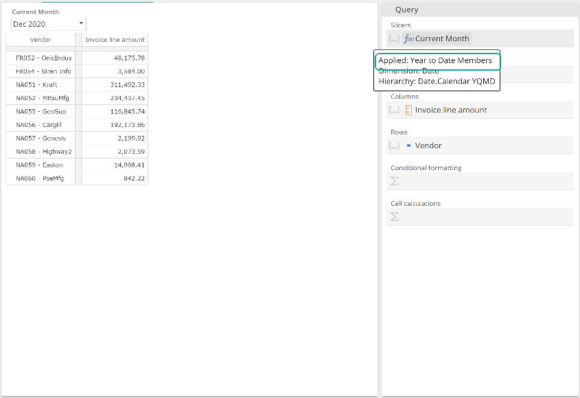
Please do note to the Invoice line amount measure is now on Columns. Now show the placeholder tab menu for Current Month and select Year to Date Members as in the following image.
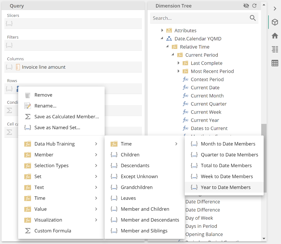 |
Selection Types are a special type of Set Function that do not wrap. Instead, you can consider that they are applied to the tab. Your table should now appear as in the following, and if you hover over the Current Month tab, you will see that the tooltip lists the applied Functions (just Year to Date Members in this case).
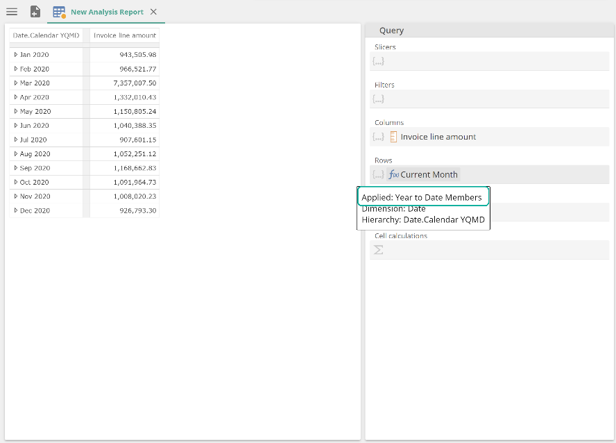 |
Because Selection Types do not wrap the inner tab, you cannot unwrap it to revert the change. Instead, you uncheck the applied Selection Types. This can be seen in the following image, but do not uncheck Year to Date Members.
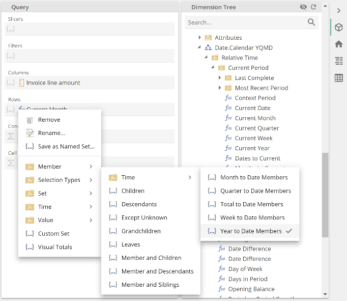 |
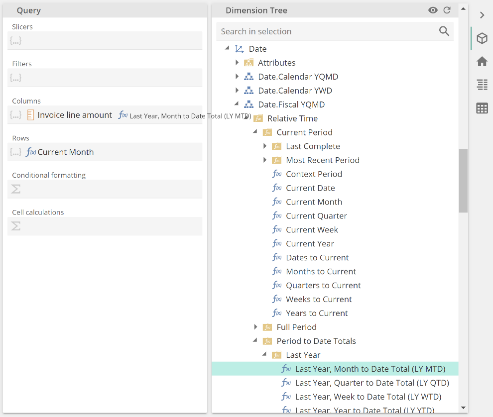
You will also see there are non-Time selection types. However, the Time folder selection types are more commonly used. We will return to discuss this topic a little further in a later section. Back to the design at hand, show the placeholder menu for the Columns placeholder (right-click in the space to the right of the Invoice line amount measure). Expand the menu to locate the Last Year, Month to Date Total (LY MTD) Function, as in the following. We could also have taken this function from the Dimension Tree, but you’ll soon see why we’ve taken this route.
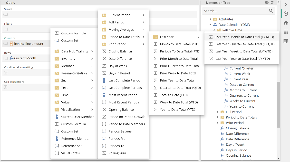 |
Recall you can hover over any Function for a description. We’ve not elected to do so in this image, as the tooltip would have overlaid the menu. The name of the Function gives us a reasonable understanding of what it will do, and do note the Sigma (Σ), which indicates it is a Value Function. So we would expect this Function will, using its Time Member field as the reference point, return the same period in the last (previous) year, and then with this period, perform a month-to-date total for a given formula. That’s a little to take on, but our table has months on rows (not dates). So we can simplify the previous statement for our scenario to using its Time Member field as the reference point, the function will return the same month in the last (previous) year, and for a formula.
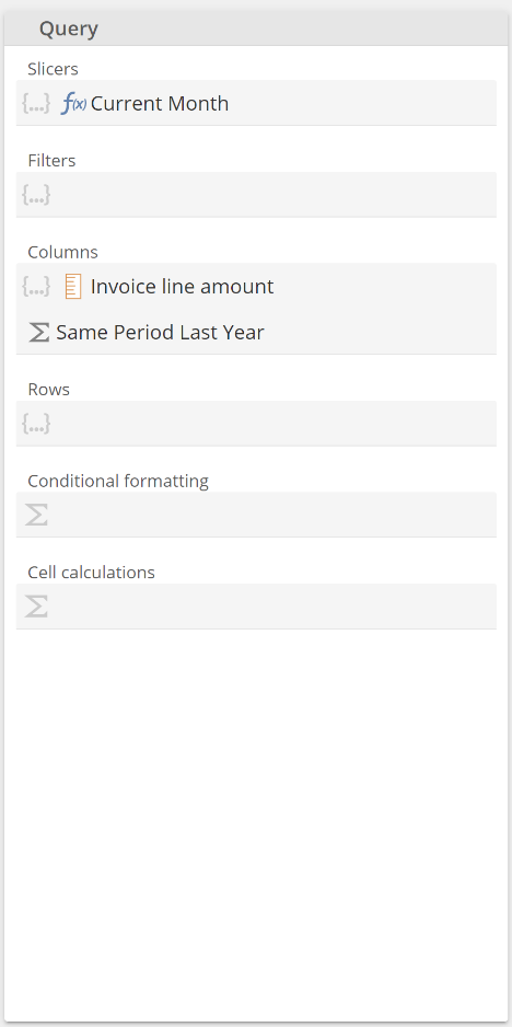
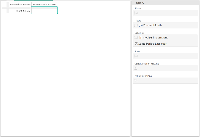
Select the Function so we can see how we will configure this. Our existing column is Invoice line amount. So drag Invoice line amount from the Columns placeholder to the Formula to aggregate placeholder, and we’re done. Remember, we are intentionally leaving the Time member placeholder empty. It’s worth renaming the function to Same Period Last Year. The result should be as follows.
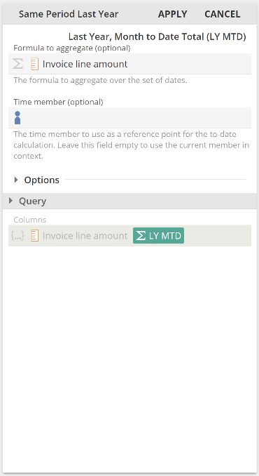 |
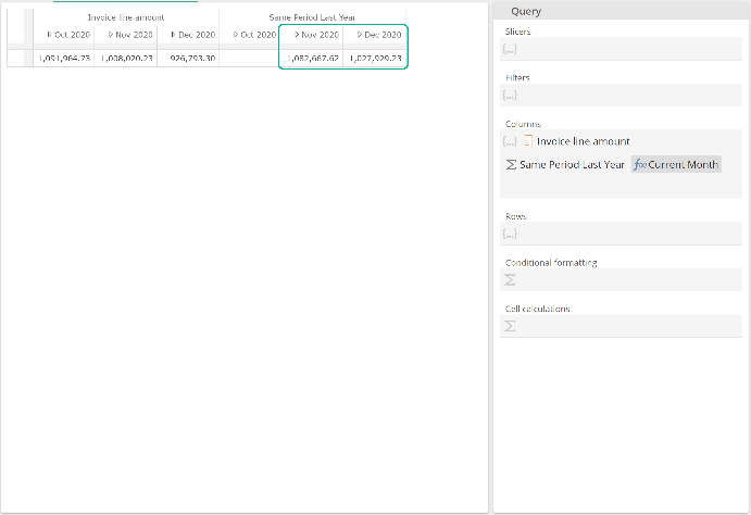
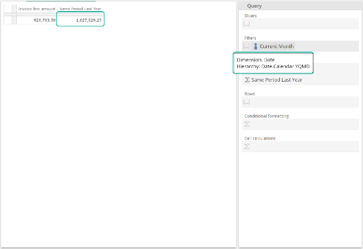
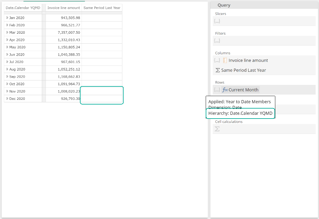
Click Apply and the table shows the amount of the invoices for the same periods in the previous year.
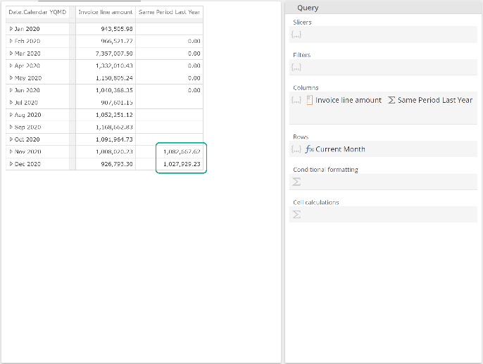 |
By leaving the Time member placeholder empty, each evaluation of the Same Period Last Year function must now determine a time context from its position within the table (we’ll expand on this shortly). Time context is the Date-hierarchy context provided to each evaluation (each cell). So put simply, each Same Period Last Year cell requires time context. Let’s take the first row (Jan 2020). There are two cells within this row, one for Invoice line amount and one for Same Period Last Year. For both of these cells, the time context is Jan 2020. Obviously, the Invoice line amount cell of the first row doesn’t require time context, but it receives time context nonetheless. Given that the Same Period Last Year cell receives the Jan 2020 time context, we have satisfied its requirement. This cell can now use that period to generate a value for the Same Period Last Year, which will be Jan 2019.
Let’s now mix the table up a little. Take the Current Month tab (with Year to Date Members applied) and drag it to rows before the existing two tabs. The result should be as follows.
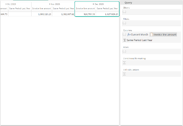 |
We’ve scrolled to the table to the far-right in this image because there are now many columns, but importantly you can see the same values as from the previous table. Although you can’t see it from this image, all values are identical. In this example, we can see each Same Period Last Year cell is now able to determine its time context from the outer row header. Now drag the Same Period Last Year tab to after the two other tabs. The result should be as follows.
 |
It’s worth noting we’ve changed the Current Month Selection Type to Quarter to Date Members to see the overall table format. Again, you can see the same values as from the original table. In this example, we can see each Same Period Last Year cell is now able to determine its time context from the outer row header.
We can take this further. We initially introduced the fact that context is determined by a cell's position within the table, and we promised to expand on that point. So let’s now move the Current Month tab to the Slicers placeholder, as in the following image.
 |
As we step the available slices, we will see our <> values are maintained.
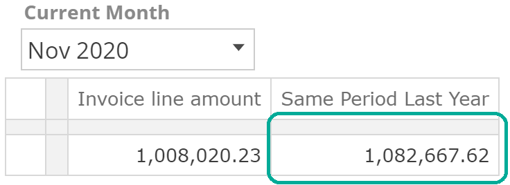 |
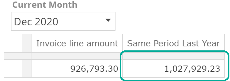 |
In this example, we can see each Same Period Last Year cell is able to determine its time context from the Slicer. It's possible to take this example one step further by removing the slicer from the Analysis Report and providing the same slicer on containing dashboard. We’ll talk more about dashboard slicing in the future Dashboards section. Let’s now try the Current Month function (with Year to Date Members applied) to filters.
This time we’ve lost our values. The Current Month function (with Year to Date Members applied) does not provide time context because it is a set of months. Time context must be a member, not a set. We can resolve this by unchecking the applied Year to Date Members Selection Type.
 |
From this image, note that Year to Date Members is no longer applied to Current Month, so the Filter placeholder is now providing a single member for Context (Dec 2020). And yes, this table could do with a title or dynamic captions.
What we’ve just stepped through demonstrates the sole differentiator of Time Functions from all other functions. That is, Time Functions have an optional Time Member placeholder that will be substituted at evaluation time for a time context member. That’s it, you now understand Time Functions. In all other respects, Time Functions behave as any other Function would.
There are, however, a few more options we might use to populate the optional placeholder. So far, we’ve seen we can specify a member or leave the Time Member placeholder empty. By leaving the placeholder empty, we tell the function that it may pick up any Date-hierarchy member. What this means is that, where previously, we have been using the year-to-current months on rows from the Date.Calendar YQMD hierarchy, we could easily swap across our rows to year-to-current months from the Date.Fiscal YQMD hierarchy. If our financial year runs July-June, then the table will be quite different, but we don’t need to change our Same Period Last Year Function definition in any way. The following screenshot demonstrates this.
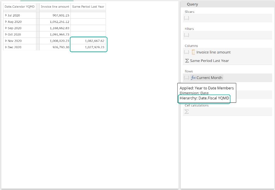 |
This should emphasize just how flexible Time functions are. But what if a report makes use of two Date hierarchies? For example, a report may make use of an Invoice Date and a Shipped Date hierarchy. In such a case, it is possible to restrict a Time Member placeholder only to accept time context from a given hierarchy. This is achieved by populating a Time Member placeholder with a hierarchy. In the following image, we’ve elected to restrict the Same Period Last Year time context to the Date.Fiscal YQMD, presumably because we will make use of another Date hierarchy as we built out the query design.
 |
However, with this restriction in place and with the Date.Calendar YQMD month members on rows, the Same Period Last Year cells are no longer able to determine time context.
 |
This example nicely demonstrates that restricted time context may result in empty cells, while unrestricted time context may result in incorrect cells (did you require the same period last calendar year or last fiscal year?). For this reason, it is best practice to restrict time context to a specific hierarchy unless your query design explicitly requires the flexibility provided by an unpopulated Time Member placeholder.z
To summarise, Time Member placeholders will seek out any time context unless they are populated with a hierarchy. In such a case, they will then only accept time context from the matching hierarchy. This is our opportunity to tie off a loose end. Recall when we added to Same Period Last Year to Columns, we did so by selecting the Last Year, Month to Date Total (LY MTD) Function from the placeholder menu and not from the Dimension Tree. The reason being, each Time Function on the Dimension Tree is under a hierarchy item, and when dragged from the Dimension Tree, the Time Member placeholder of the Function will default to that hierarchy. To see this, let’s right-click Remove the existing Same Period Last Year Function then replace it with Last Year, Month to Date Total (LY MTD) taken from the Dimension Tree under the Date.Fiscal YQMDhierarchy. The following image shows the Columns placeholder immediately before dropping the selected Function.
 |
The result of dropping the (now) LY MTD Function on Columns is shown in the following, and note we don’t see the placeholders for LY MTD. This is because all the placeholders for LY MTD are optional.
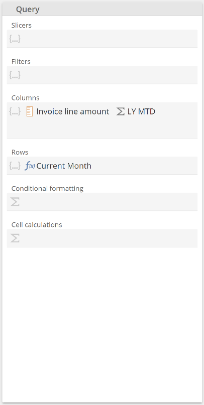 |
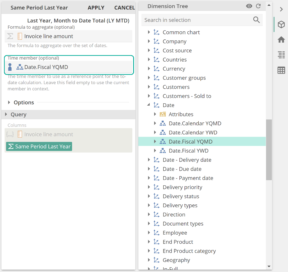
Click on LY MTD, and now we see that indeed the Time member placeholder has defaulted to the hierarchy from which we dragged the Function.
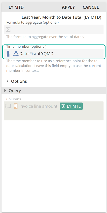 |
We’ll talk to optional Formula placeholders shortly. They are not unique to Time Functions. Suffice it to say that you want to populate the Formula to aggregate placeholder with Invoice line amount, or it won’t provide a same-period-last-year comparison for Invoice line amount (it will actually do something quite interesting that we will need to discuss).
We’re on the Dimension Tree, so let’s discuss the Current Period folder of Time Functions, which are slightly different from all other Time Functions. They have a Time hierarchy placeholder instead of a Time member placeholder, and this placeholder is not optional. This is an exception to our previous over-simplified rule that Time Functions have an optional placeholder that will be substituted at evaluation time. This is, however, a simple exception and only for the functions from this folder.
We’ve already been making use of a Current Period function. It’s sitting there on Rows. So let’s click it now to see the query design Current Month.
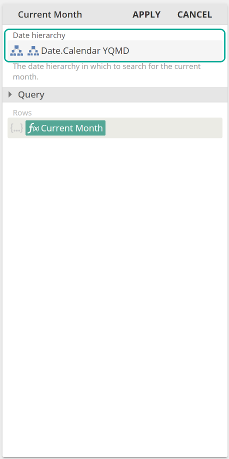 |
It should be obvious why the Date hierarchy is not optional. That is, the whole purpose of the Current Month Function is to provide the current month member for a given hierarchy.
So far, we’ve looked at Current Period functions and Period to Date Total functions. We did also see the Time Selection Types folder. Let’s put these three Time Function types into three different categories and introduces two new types at the same time
Current Period – return a member or set based on the current date. The hierarchy field is not optional.
Period to Date Totals – return a value based on the sum of periods to a given reference point
Selection Type – return a set. Selection Types are applied to a tab instead of wrapping it.
(NEW) Context and relative-context – return a member that is either the time context (as it the case for the Context Period function) or a member relative to the time context (, for example, Year which will return the year member of the time).
(NEW) Time Utility – a collection of general Time utility Functions, for example, Days in Period.
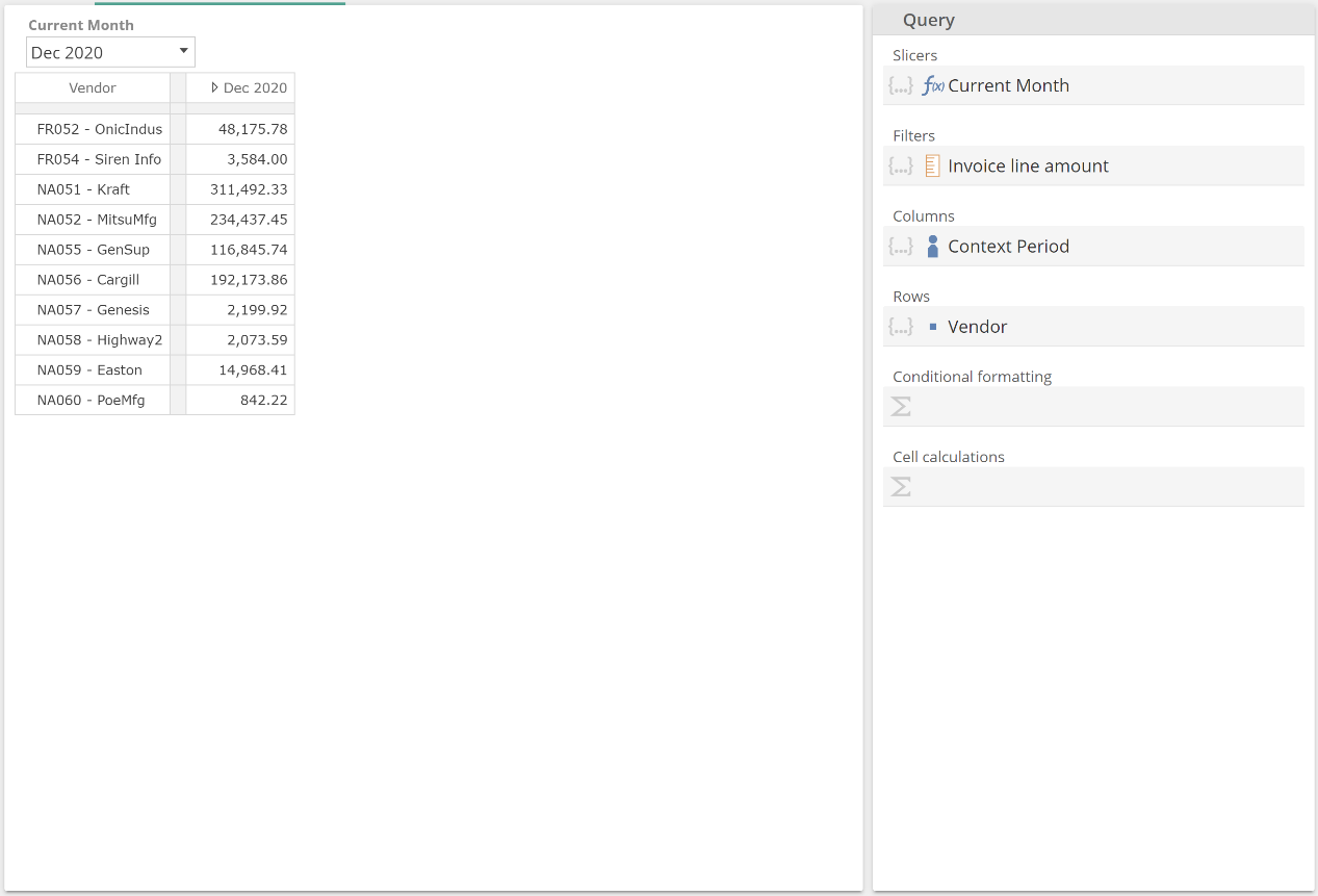
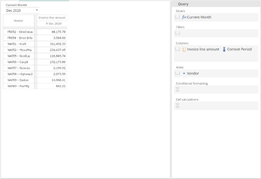
We won’t discuss the utility Functions further, as you will find them easy to use when required. It is suggested that you take a minute to review the application's available options. It is, however, very important that we discuss the context and relative-context Functions as this will complete your knowledge of Time Functions and enable you to satisfy any overtime analytic requirements. Let’s start with the Context Period. Setup the query design for a new Analysis Report as follows:
 |
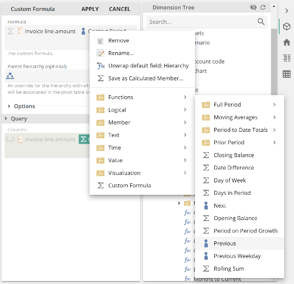
Given our table has a Slicer, the Invoice line amount column shows values for the selected month. Our requirement is for an additional column to the right with the previous month’s values. Notice from the image that the Slicer is providing Date.Calendar YQMD. We now drag Context Period from the Dimension Tree, from under the Date.Calendar YQMD, across to the Columns placeholder. Before we apply the Previous function to the Context Period, let’s first look at the table.
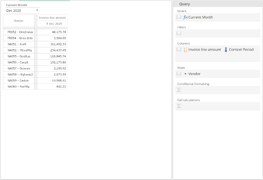 |
This certainly isn’t satisfying our requirement. Instead of introducing a second column to the table, we’ve introduced a second column header. Recall from our fundamentals that same-hierarchy sets are appended, and different-hierarchy sets are combined (each member of the first hierarchy is combined with each member of the second hierarchy, in a two-hierarchy example). Keeping in mind that a single member or measure is treated as a set, this statement tells us we require our two tabs to be the same hierarchy to add (append) a second column.
However, our Columns placeholder now includes members/measures from two different hierarchies. And so, each measure from the first set (the single Invoice line amount measure) is combined with each member from the second set (the single Context Period member). In this sentence, we’ve stretched the definition of a hierarchy slightly to consider measures as also existing within their own special hierarchy. The result is that our single measure is combined with our single member to produce the single column. Let’s quickly resolve this issue to make the point clearer, and then we’ll leave the topic of hierarchy-grouping for the next section.
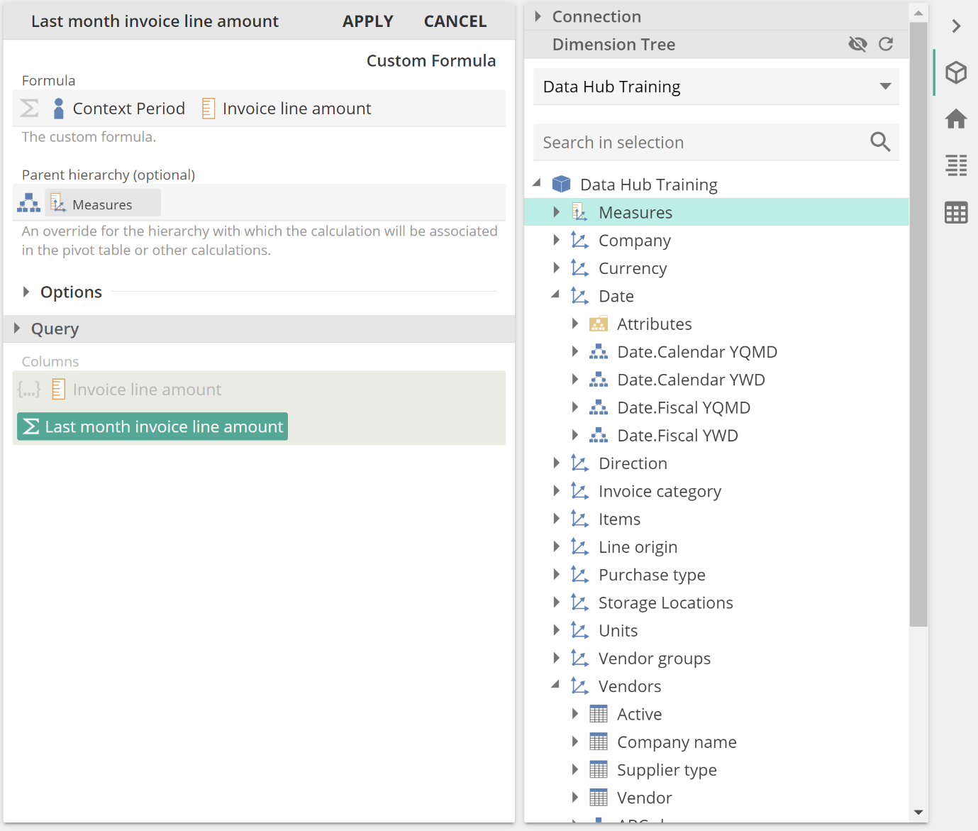
Right-click on the Context Period Function and select Custom Formula and drag the Invoice line amount measure to the left of Context Period in the Formula placeholder. You can pick up the Invoice line amount from the Dimension Tree or the Columns placeholder.
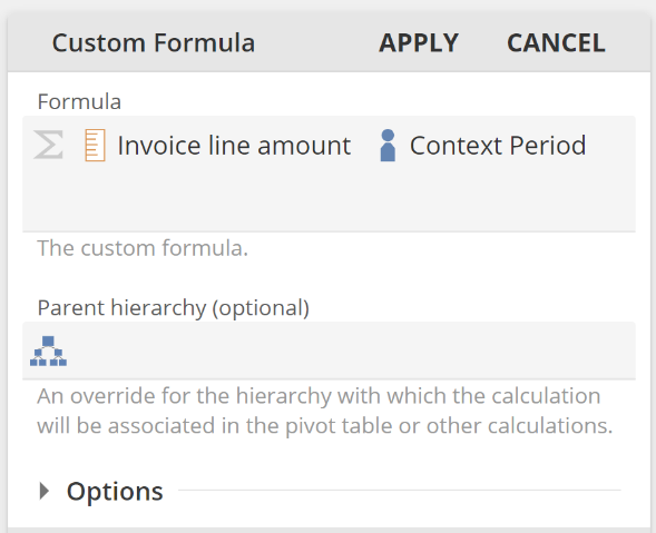 |
Click Apply at this point, and we now have a second column.
 |
And the reason is that our second tab is now from the Measures hierarchy, as we can see from the following image.
 |
That was a little magic, as we’ve not yet provided the reason that Custom Formula is now a measure (a calculated measure, which we’ll talk to again). Click on the Custom Formula function from Columns open it for edit again. Recall the emphasis on placing the Invoice line amountto the left of Custom Formula? The importance of this is that the first tab in a Formula placeholder (where one exists) provides the hierarchy of the Function. So tracing it through, by merit of Invoice line amount being the first tab, Custom Formula becomes a measure. By merit of it being a measure, the Columns placeholder now has two measure tabs. And by merit of the same-hierarchy-sets-append rule, these two tabs now result in two columns. Please do take your time to be completely comfortable with this explanation. It is one of the more important concepts for building our more complex analytics.
Finally, the only step remaining to achieve our end goal is to apply the Previous function to the Context Period Function.
 |
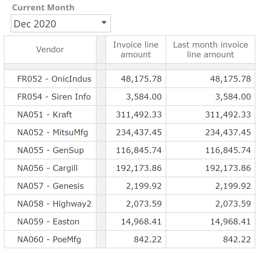
It’s worth noting that the Previous and Next functions are applied, as with Selection Types. They are, however, not Selection Types because they each return a single member. Rename the Function and click Apply. The final result is shown below, and we’ve resized the columns so the header text wraps.
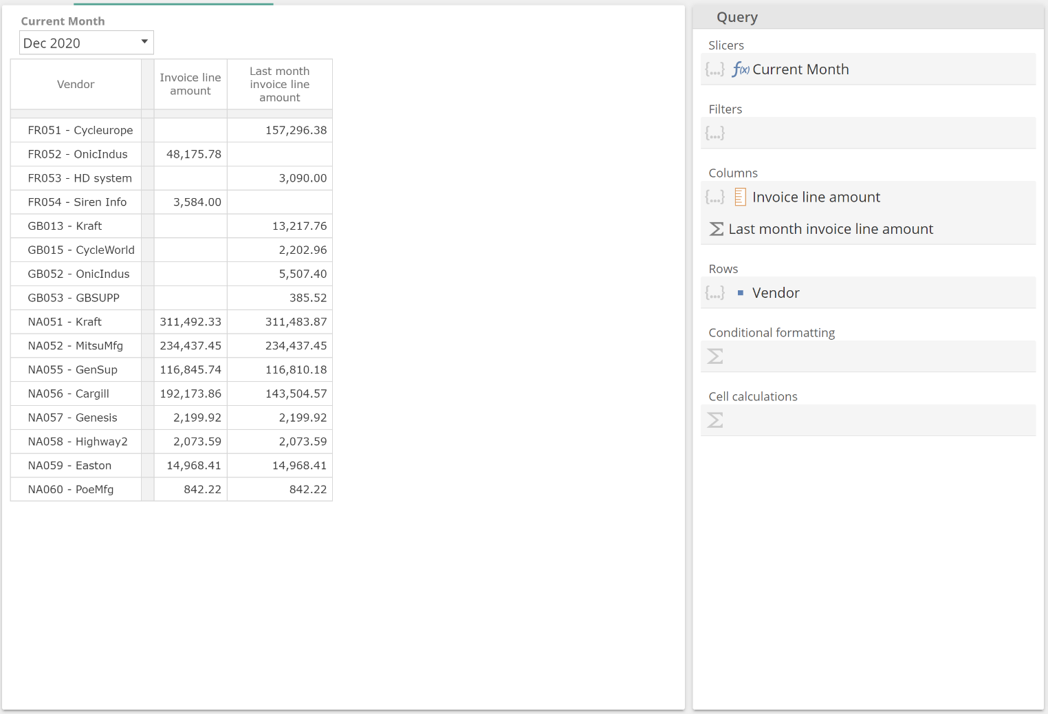 |
If you look closely at the data, you will see some vendors have the same invoice amounts for both the current and the previous month. Presumably, a recurring monthly order is in place. At this point, you may observe that the Slicer selection is Dec 2020, but the Last month invoice line amount column is, by definition, showing Nov 2020 values. This is important. Slicers slice members but notvalues. Custom Formula is a Value Function and, for this reason, is not affected by the Slicer selection.
Now let’s quickly rebuild the same report in a different format so we may talk about the interplay between time context and Slicers. Configure the query design as follows (with Year to Date Members still applied to Current Month).
 |
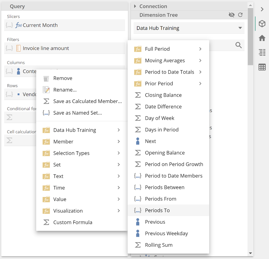
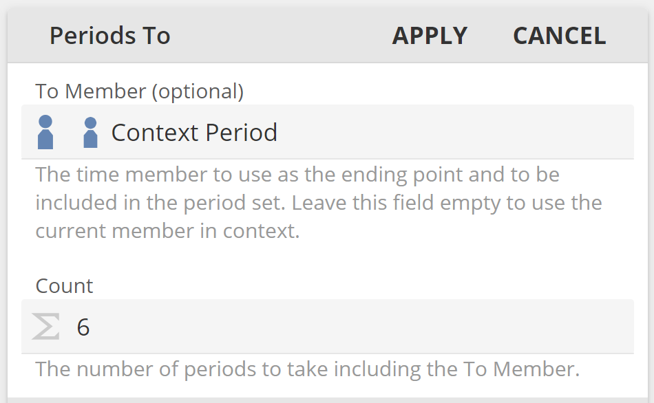
In this example, we now have the measure in the Filters placeholder. The reason for this is that our requirement is to now show the six months up to and including the Slicer selection. It would be onerous to create five calculation in the manner shown (and note in such a scenario the additional columns would need to make use of the Lag/Advance Function instead of the Previous Function). The alternative is to have the Columns placeholder provide a set of months. For this, we right-click Context Period and select Periods To, as in the following.
 |
Because the Set Function names don’t reflect on the table, we’ll leave it as it. Enter 6 for the Count and click Apply.
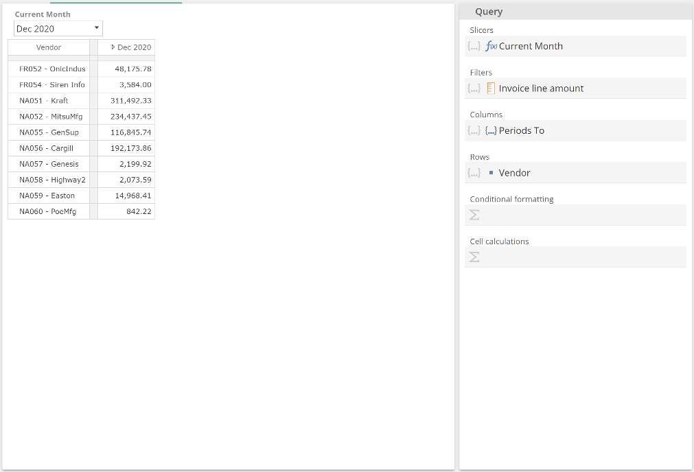 |
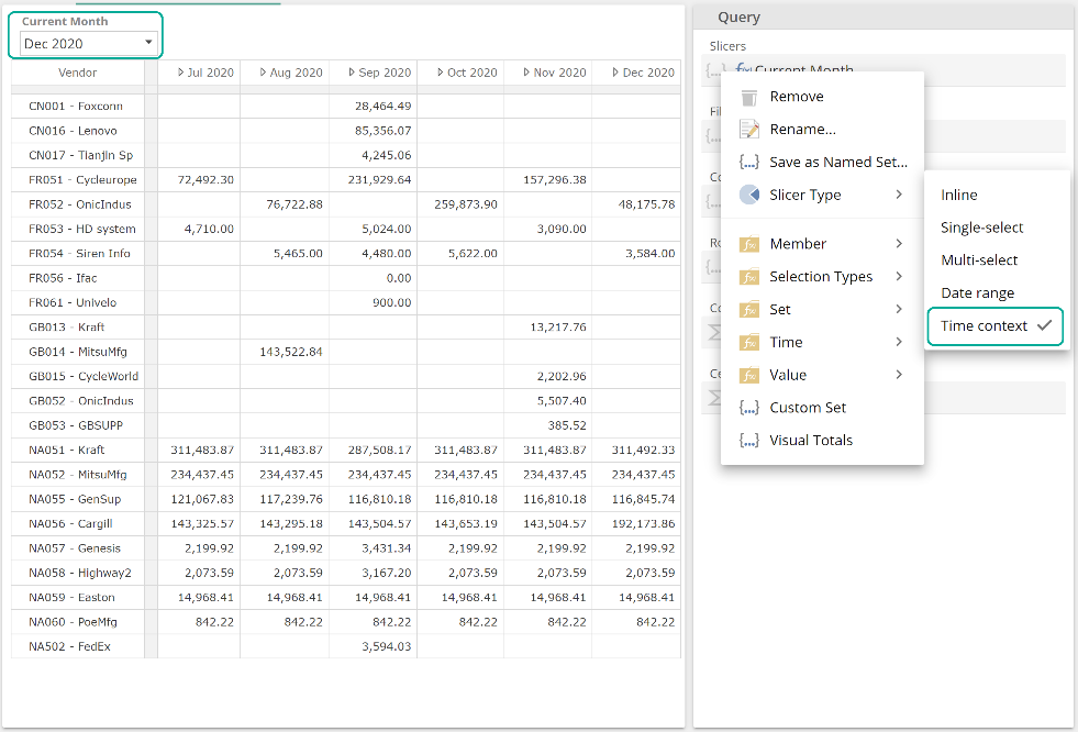
Well, that didn’t work. Recall Slicers slice members (sensibly), and we now have month members on Columns. The result is that the Slicer has a detrimental impact on our table. We can resolve this by changing the Slicer type to either Date range or Time context. Let’s start with the Date range Slicer type. Recall you change the Slicer type by right-clicking and selecting a type from the placeholder tab menu, as in the following.
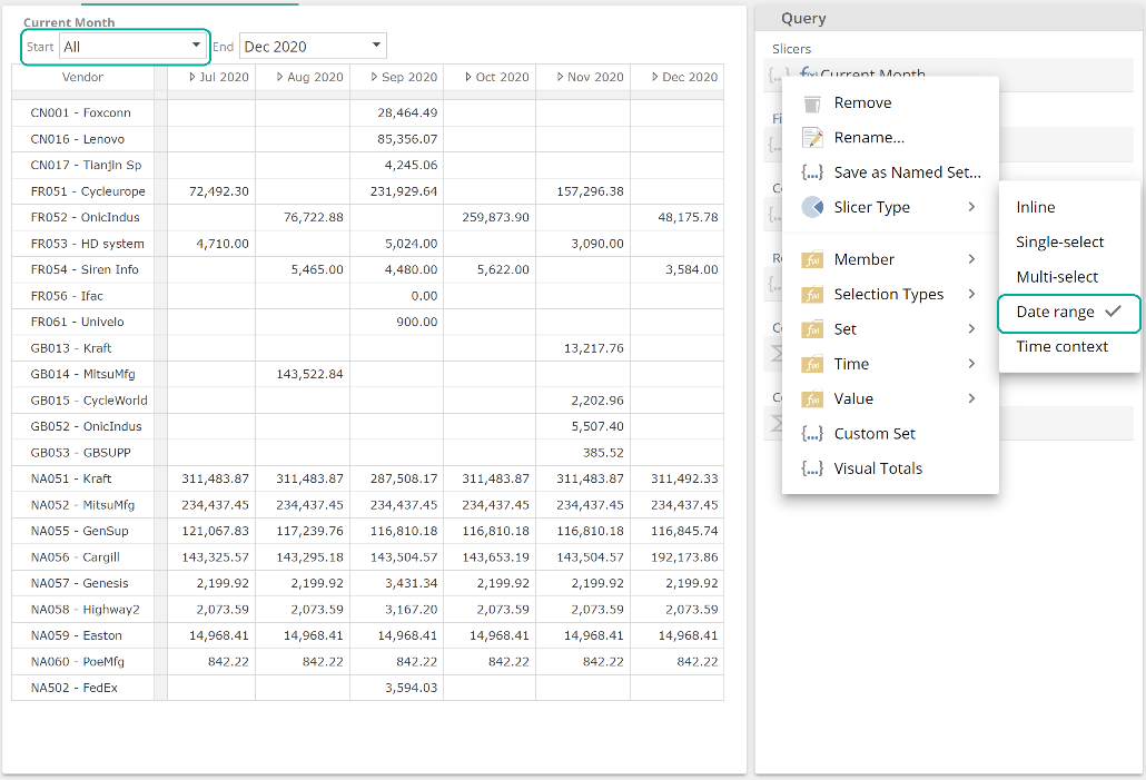 |
From the image, you can see there is now an additional Start drop-down to select the starting member (or All, as in this case). Keeping in mind we configured the Periods to Function to return six months (inclusive), you can now see July through December across the columns. This is because our Slicer is slicing for the range of all-members-to-Dec 2020, and importantly, the End drop-down is providing the time context for the Context Period function. So the table now satisfies our requirement, but the Slicer now arguably includes a superfluous drop-down.
A better approach to this requirement is to use the Time context Slicer type (assuming the Date rangeStart drop-down isn’t serving a purpose). Consider that the default Single-select Slicer type both slices members and provides time context. You might then correctly guess that the Time context Slicer only provides time context. If we change the slicer type now, the result will be as in the following image.
 |
We can see the table is unaffected because the new Slicer type is not strictly slicing but provides time context. This behavior ensures we continue to see the six-month members to Dec 2020, and we’ve also saved on the superfluous Start drop-down.
There is just one minor point to be made here. In building the current query design it was convenient to right-click on the Context Period tab to wrap it in Periods to. The result was the following.
 |
The Context Period function is returning the time context member for the Date.Calendard YQMD. We know this because we took it from under the Date.Calendard YQMD hierarchy on the Dimension Tree, but we can also hover over the tab to get its hierarchy, as in the following.
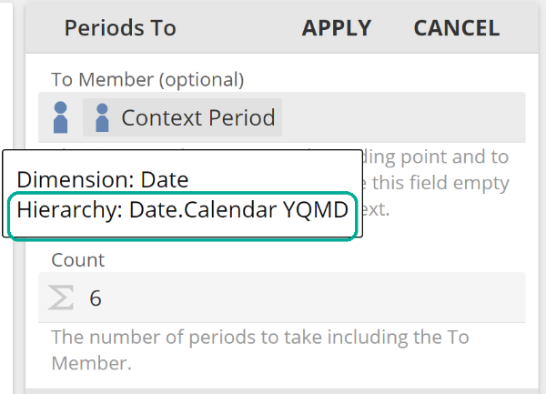 |
However, by this point, you will be familiar with the fact that a Time Member placeholder is optional, and moreover, by populating it with a hierarchy, it will only seek time context from that hierarchy. That is, the following query design is equivalent.
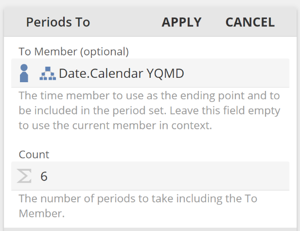 |
So it is never necessary to place a Context Period function in a Time Member placeholder, but nor is it an issue, should you find you do so in the process of building out your query design.
This completes our discussion of Time Functions. It is recommended that you take some time to familiarize yourself with the Time Function library, but let’s just quickly take a look at the commonly used Time Function and Time Function groups.
Context Period – a powerful Time utility Function, as seen in previous examples.
Current Period – for example, Current Month or Months to Current.
Period to Date Totals – for example, Year to Date Total.
Selection Type – for example, for Year to Date Members applied to the Context Period Function
Prior Period – for example, Context Period wrapped in Period in Prior Year to provide the same month (say) from the prior year.
Next, Previous (and Lag from the Member Folder) – for example, Next applied to the Context Period Function.
Commonly used functions
From the commonly used Time Functions, let’s now review the commonly used non-Time Functions and provide some examples in order to give you just a little more familiarity with Functions. By this point, you’ll be familiar with the Custom Formula Function, as in the following image.
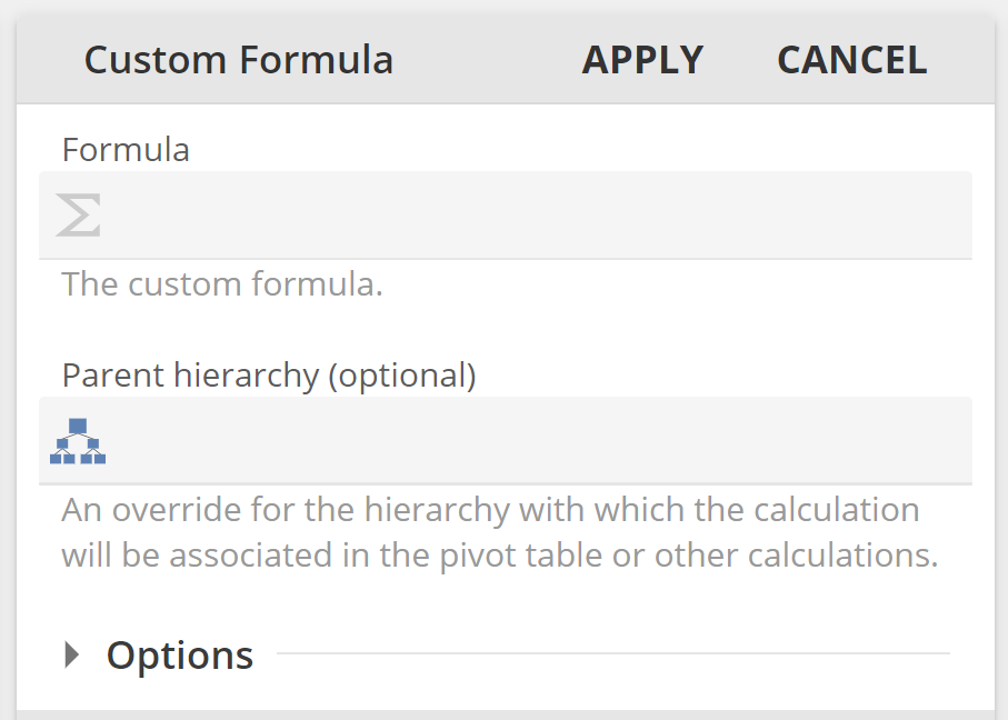 |
We’ve already seen Custom Formula as the basic go-to Function for entering formulas. We will talk to the Group-by hierarchy placeholder in the next section. We will also talk to the common Options area later in this article, so for now, let’s move on.
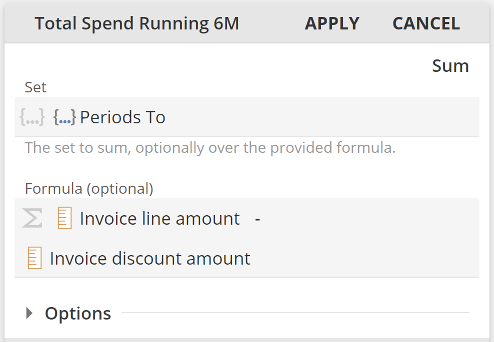
The Sum Function is a natural complement to the Custom Formula function in that it also evaluates a formula, but it does so for each member of a provided set, summing the results as it goes. Importantly the Formula placeholder is also optional. Based on this description, sensibly, the Sum function is also of the Value type (returns a value, not member or Set). The fields of the Sum Function are shown in the following.
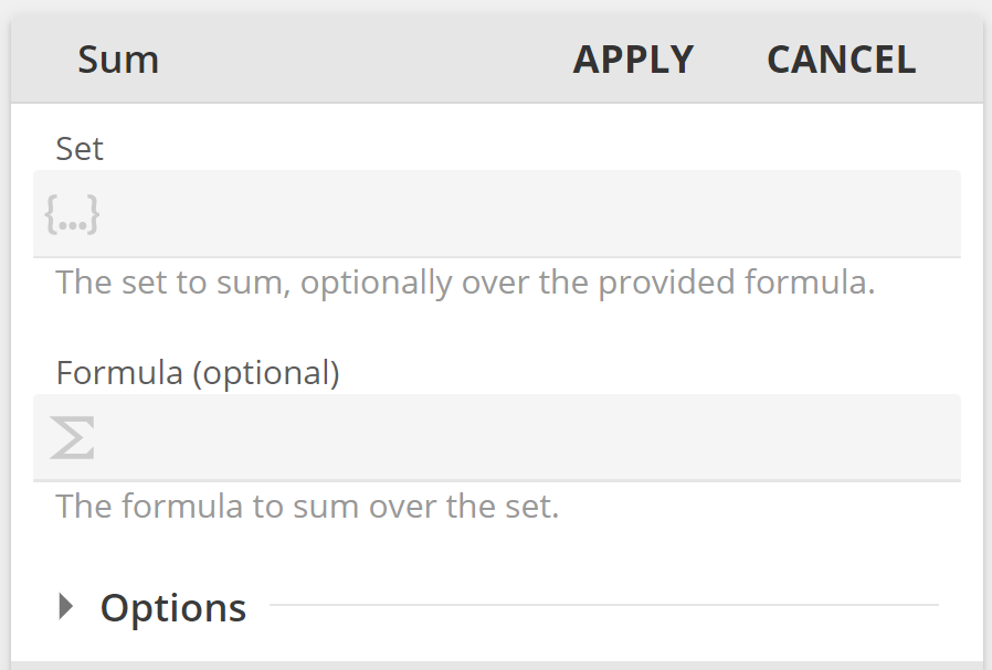 |
To demonstrate this function, let's return to the example wherein we introduced the Date range and Time context slicer types. The following example will work with the Slicer type set to any of the three types discussed (Single-select, Date range, or Time context). Recall the Periods to Function returns six months up to and including the current Slicer selection. Right-click the Periods to Function and select Sum, as in the following.
 |
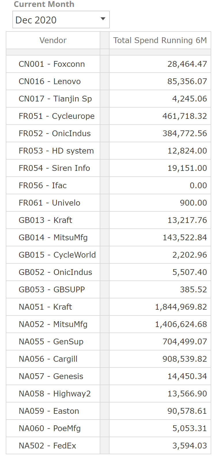
Because the Formula placeholder is optional, the query design panel doesn’t show the Sum function fields, and instead, the table reflects the change immediately, as in the following.
 |
In this example with an empty Formula, each Sum value is simply the sum of the six months to Dec 2020, for the given vendor and for the Invoice line amount measure provided in the Filters placeholder. Let’s now populate the Formula placeholder. To simplify this discussion (and in order to leave a topic aside for later), remove the Invoice line amount from the Filtersplaceholder and now populate the Sum Formula placeholder as follows.
 |
Click Apply, and each value is now the sum of the provided Formula for the six months to Dec 2020, for the given vendor. This is shown in the following.
 |
The Sum function is particularly useful for ad-hoc categorization (for example, summing a set of item types or regions). Be aware that Ctrl-clicking and shift-clicking allow multiple tab selections within a placeholder, in the same way, they allow multiple-member selection from the Dimension Tree. The following trivialized example shows the Food and Pharmaceutical tabs both selected (evident by the darker shade). Right-clicking either tab will now show all functions with a Set primary placeholder. As discussed, the Sum Function has a Set type primary placeholder and so shows in the placeholder tab menu as in the following.
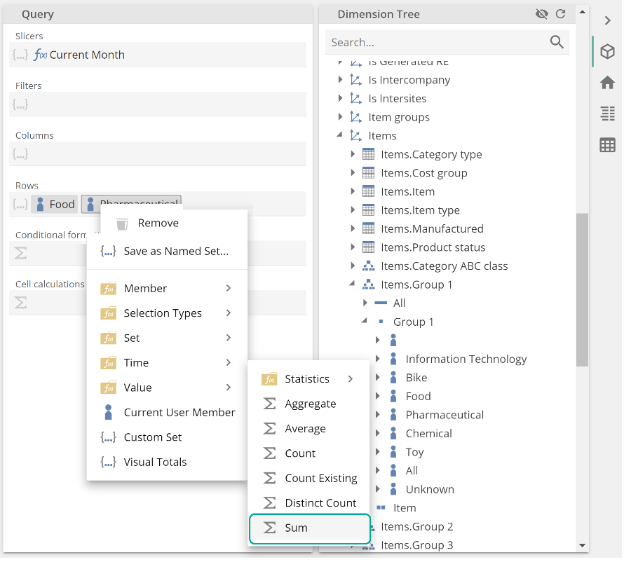 |
The Sum function is also particularly useful for summing account ranges when combined with the Range Set Function. We’ll leave this as an exercise for the reader. Finally, while this example above served us well, it is worth noting there is a Rolling Sum Function in the Time folder that packages up the Sum and Periods to combination in a single easy-to-use Function.
We’ve looked at two common Value Functions. The remaining Functions we’ll address are Set Functions. We’ve already seen the Top Count Function, and the fields for this Function are shown in the following image.
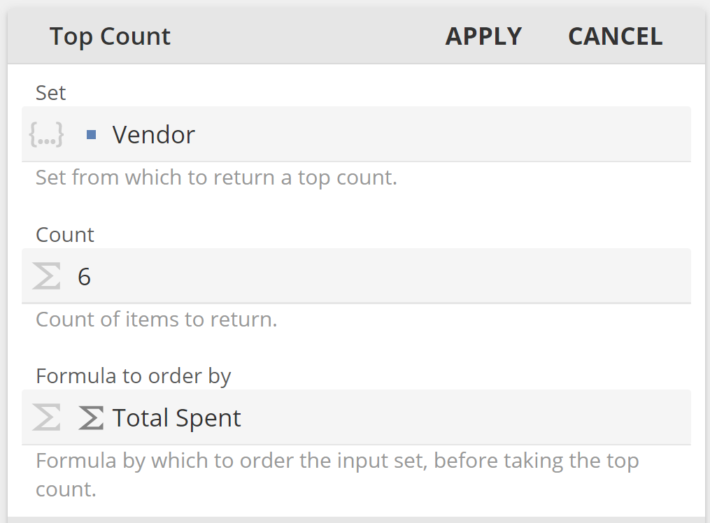 |
The Top Count function is just one of six Functions that all serve similar purposes. These functions both filter and order the members of a set. The available functions are shown in the following.
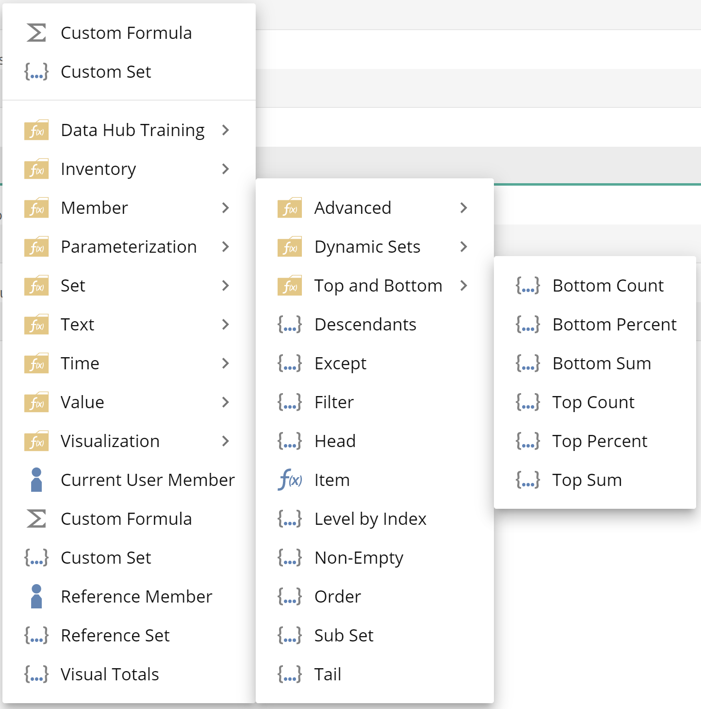 |
Let’s move on to a function that only filters without ordering the set. You might imagine we call the Filter Function. This Function introduces a Logical placeholder that must evaluate to true or false, as in the following example.
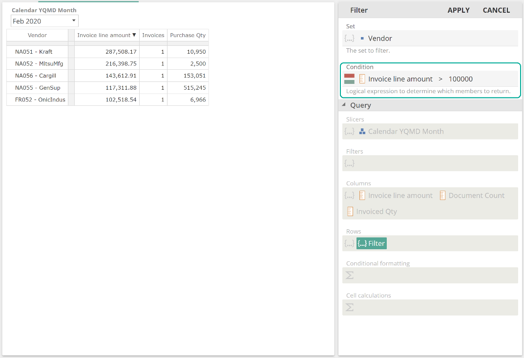 |
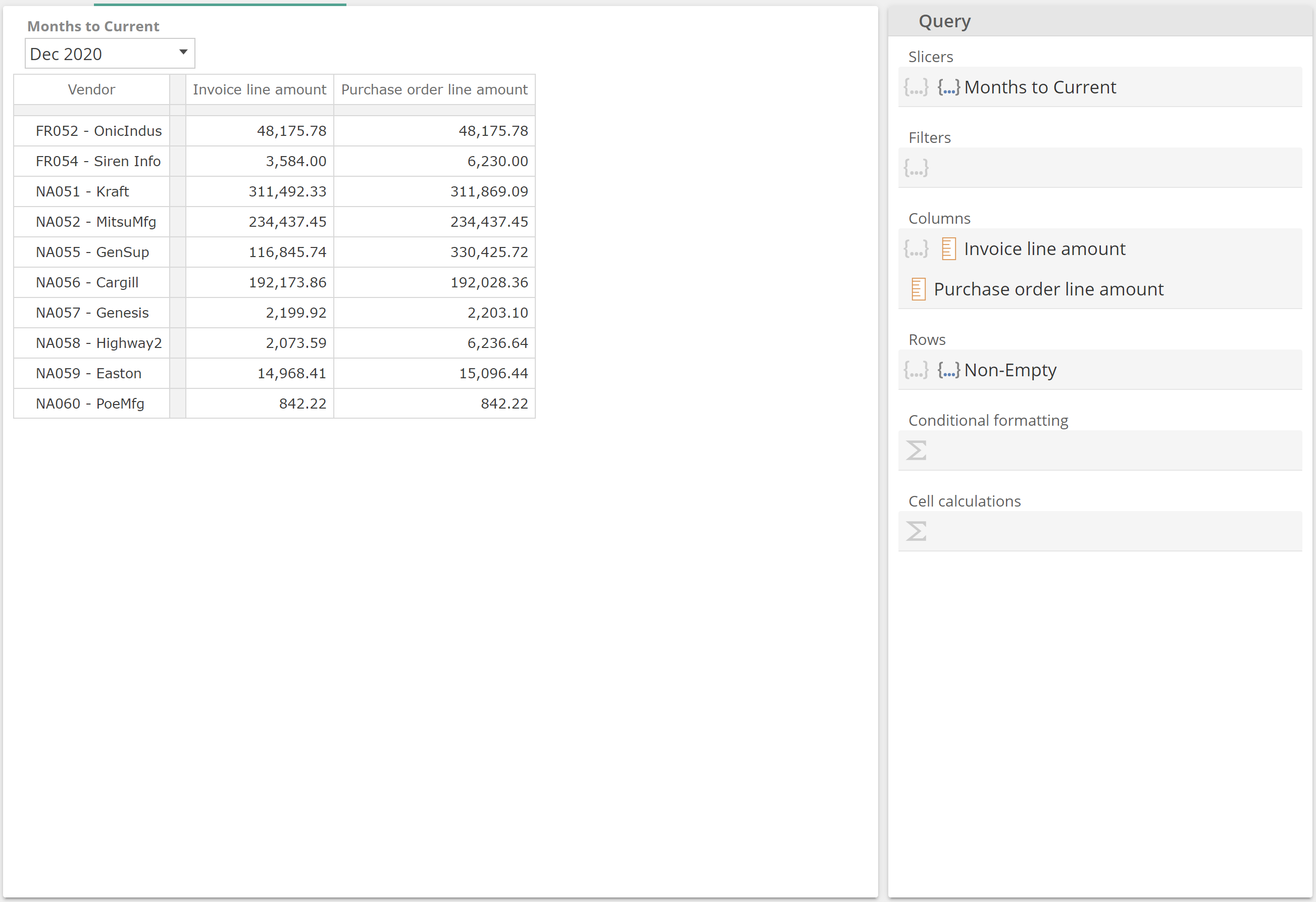
That’s simple enough. Let’s move on to the last Function we’ll discuss. It may be a stretch to say that the Non-Empty Function is commonly used, but it is important to have in your quiver. Take the following analytic.
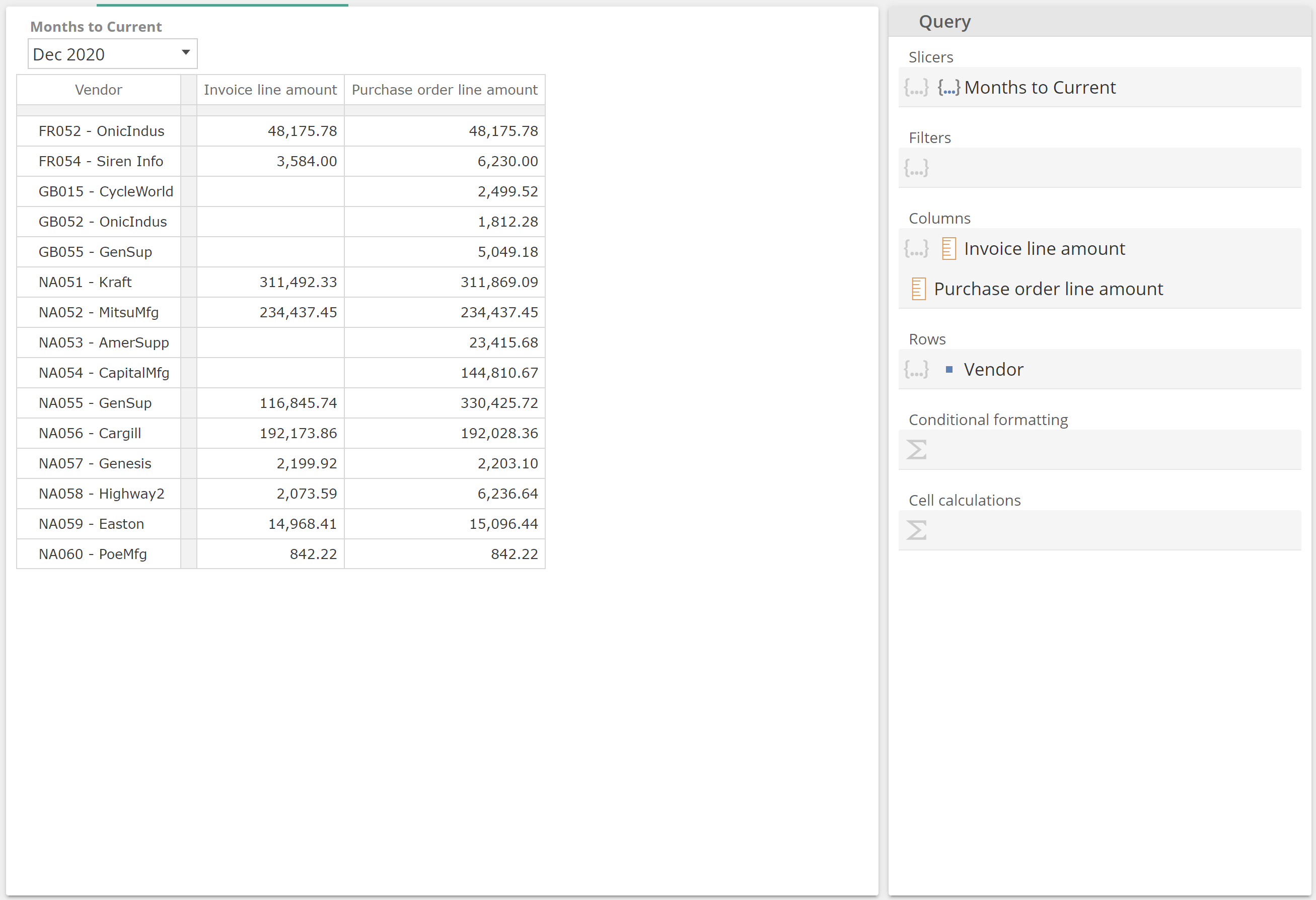 |
In this example, we’ve taken two different measures from two different measure groups by merit of introducing the Purchase order line amount measure is from the Purchase orderlines measure group. We can see that the Invoice line amount measure has far fewer values than the Purchase order line amount measure. For reasons relating to the data model and beyond this document's scope, this specific scenario only happens when we combine measure groups, which is why we called this out.
Now, if we want to show only those rows with Invoice line amounts, we will not be able to make use of the tables built-in Filter Empty Rows option (from the Data design panel). Instead, we can wrap Vendors in the Non-Empty Function in order to have this Function return only the vendors that are non-empty for the Invoice line amount Measure.
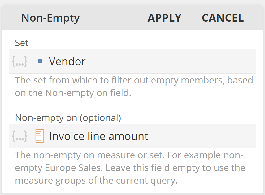 |
The result of this query design is as follows.
 |
It is worth pointing out that the Non-empty on placeholder is not limited to measures. It can also hold members and even member/measure combinations, which will be discussed further in an upcoming section.
Specialized Functions
From commonly used functions, let’s now touch on a few specialized functions to be aware of, starting with Reference Member and Reference Set. We have already encountered Reference Memberwhen we dragged Total Spent to the Formula to order by, as in the following image.
 |
When we drag a Value or Set Function from an inactive (greyed-out) section of the query design to inside another Function (as we did here), the application will automatically create a Reference Member or Reference Set Function. This Reference Member or Reference Set Function ensures that should the definition of the referenced Value or Set Function change, the referencing Function will reflect that change. Again, this all happens magically on drag-drop. However, occasionally, the required tab is not available to drag from the inactive section of the query design. In such a case, you may make use of the Reference Member or Reference Set Function directly from the placeholder menu. You then select the referenced Function using a drop-down. See the online documentation for a worked example.
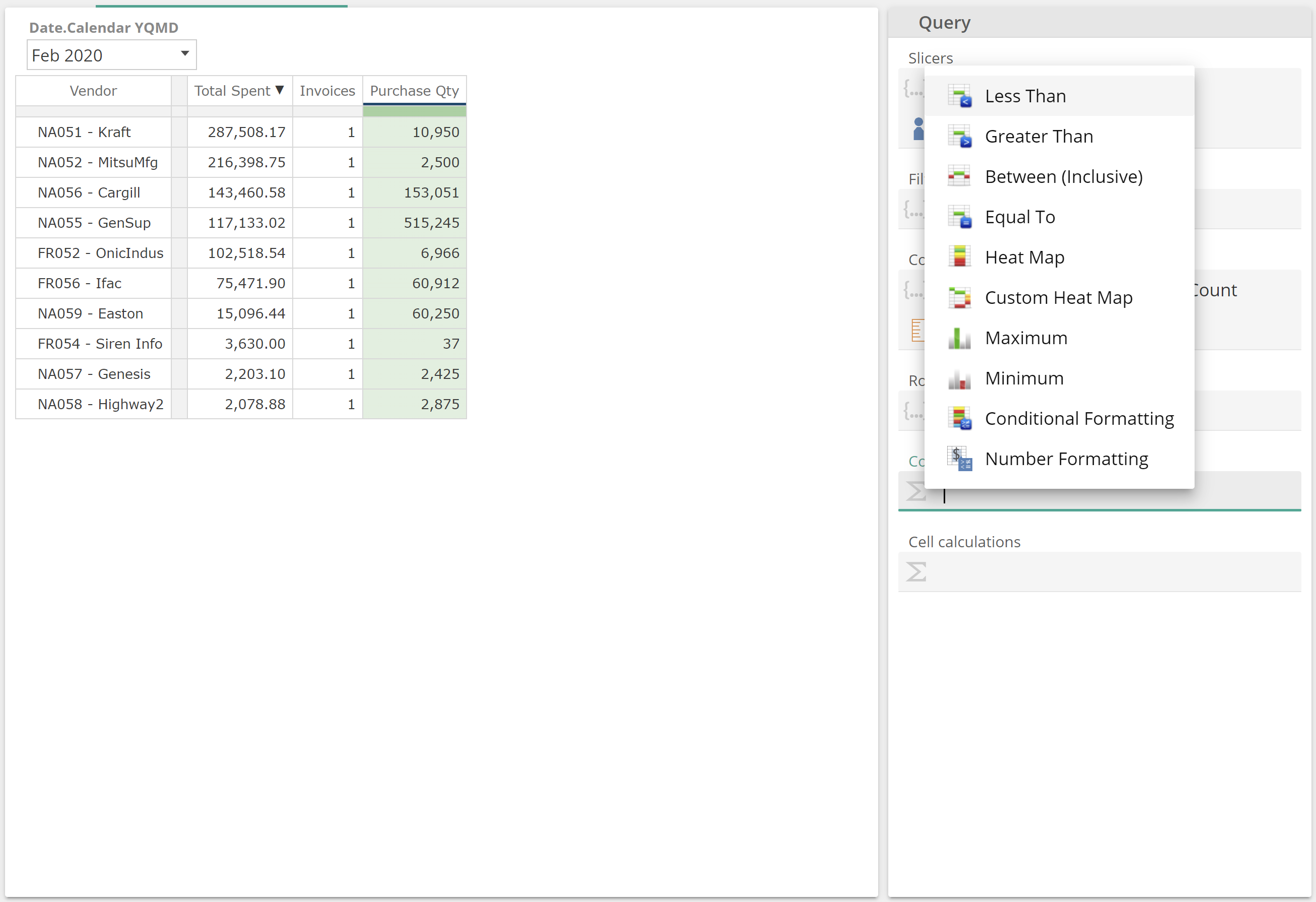
We’ve alluded to conditional formatting Functions on a few occasions to this point. Conditional formatting combines table selection functionality with Functions. Take our partial reproduction of the Top 10 Vendor Stats table from the pre-built analytics. Use the column selector and right-click to show the placeholder menu for the Conditional formatting placeholder, as in the following image.
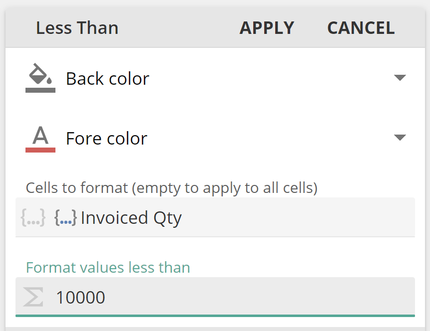 |
Enter a Format values less thanvalue.
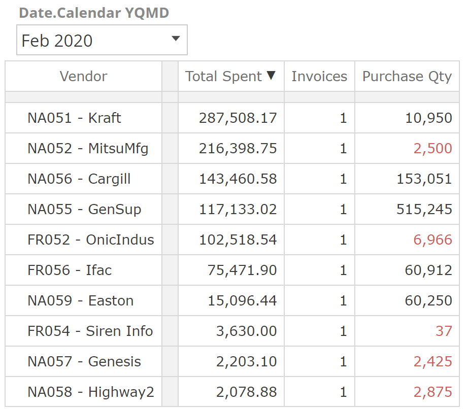 |
Click Apply, and it’s that simple.
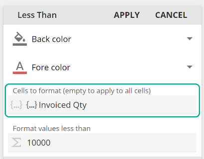 |
Or we should say it can be that simple. If we open the Less Than Function's query design, we see that the Cells to format placeholder was automatically populated for us based on the column selection.
 |
We won’t provide an example, but it’s worth being aware of complex requirements. It is possible to use Set Functions to provide the member (and member/measure combinations) that the conditional formatting rule will apply to.
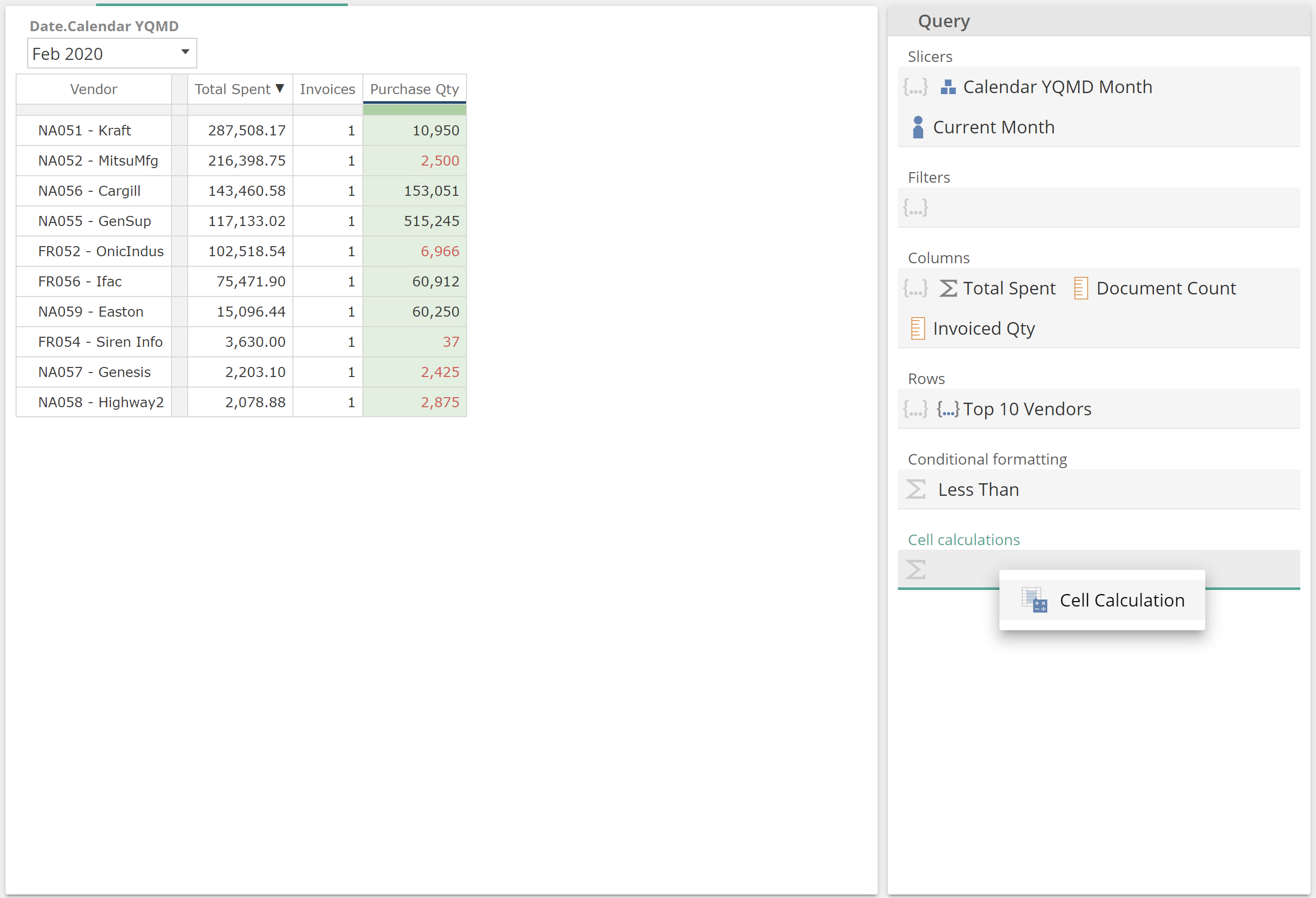
Cell Calculation Functions can be applied in the same way as Conditional Formatting Functions.
 |
Cell Calculation Functions allow you to override the value or formula for a cell or group of cells. Cell Calculations Functions are rarely required because it is usually possible to fully define a cell’s formula using the Row and Column placeholders. Should you find a need to use a Cell Calculation Function, refer to the online documentation for more information and a worked example.
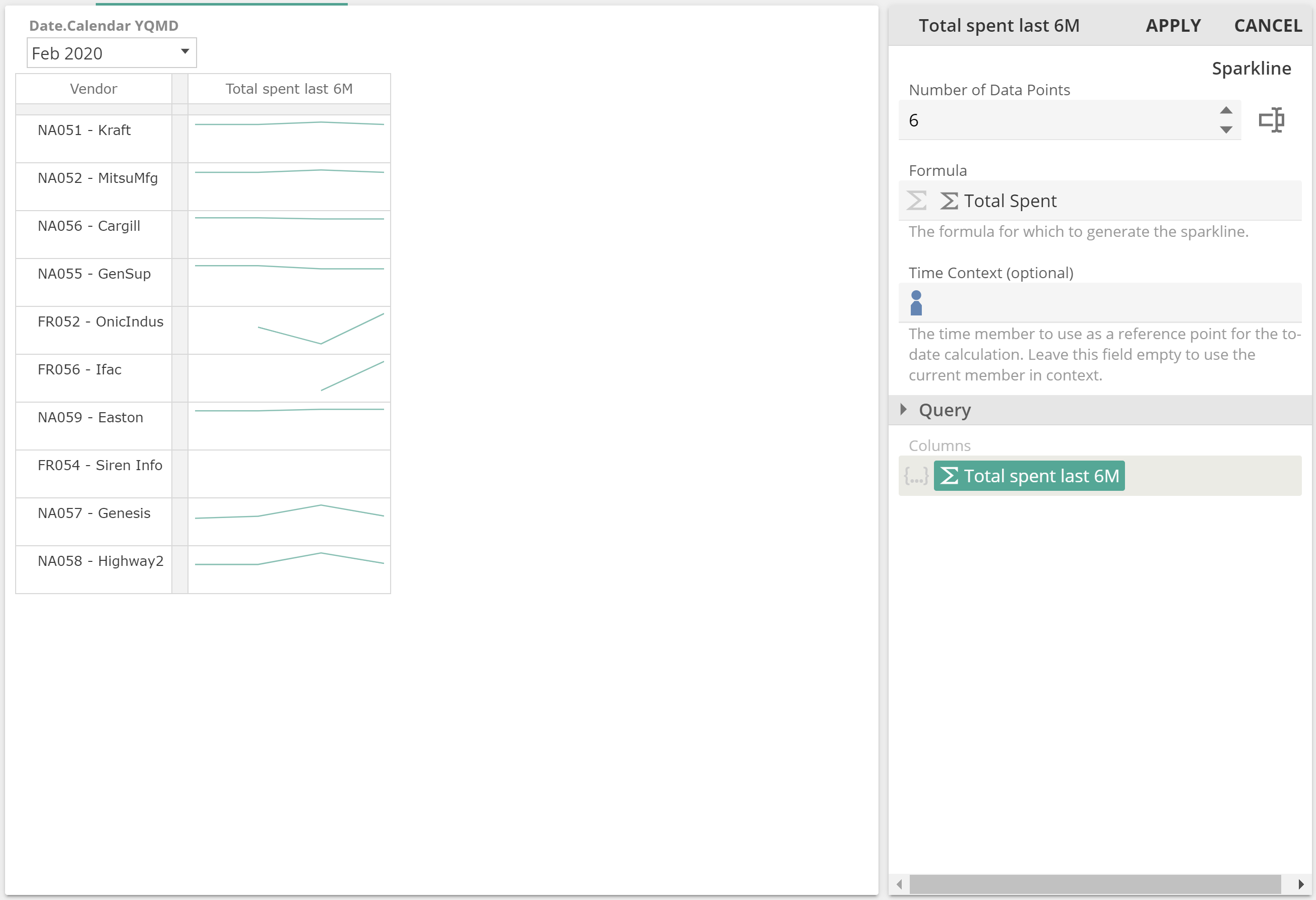
The application provides two Visualization Functions, Sparkline and Status. Visualization Functions “wrap” as we have seen previously with Value Functions. Strictly, speaking Visualization Functions are Value Functions where the value they return is the visualization for the cell. With that in mind, you should find you have all the knowledge required to make use of Visualization Functions. The following image provides a quick example of making use of the Total Spent calculation and Vendors onRows, as in many of our previous use cases.
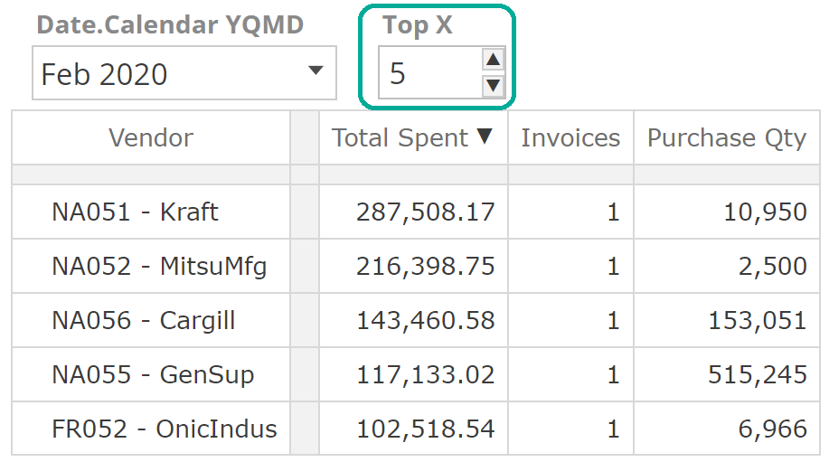 |
And finally, there are Parameterisation and Text functions. Again, both are special Value-type Functions. Parameterization Functions allow the analytic designer to provide a checkbox or textbox spinner at the top of the analytic, adjacent to the Slicers, as in the following.
 |
In this example, the count of top vendors is at the end-user’s discretion.
Text Functions quite simply return text instead of numerical values. The most used of these is the Current Members Function that returns the captions of the current members (usually Slicer selections). As with previously Functions from this section, please refer to the online documentation should you require further guidance Parameterization or Text Functions
Hierarchy-grouping for Functions
To this point, we already introduced hierarchy-grouping and seen two examples of it. We need to cover off two function topics that relate to hierarchy-grouping. To start with, recall from our fundamentals that hierarchy-grouping referred to the behavior that same-hierarchy sets are appended and different-hierarchy sets are combined.
With that in mind, let's also refer back to our second encounter with the topic. We say that the following query design resulted in the Invoice line amount measure being combined with the Dec 2020 member. This makes sense given what we know of hierarchy-grouping, given we treat measures as existing within their own special hierarchy.
 |
Our solution was to place the Context Period Function in a Custom Formula, and we emphasized the importance of the Invoice line amount being first in the Formula placeholder so that the Custom Formula would be treated as a measure.
 |
It may not be possible for more complex formulas to ensure a member/measure from the required hierarchy is first in the Formula placeholder. In this scenario, we can make use of the Group-by hierarchy placeholder. As the placeholder's name implies, this placeholder requires a hierarchy from the Dimension Tree. The following image shows hierarchy items from the Dimension Tree.
 |
However, keep in mind there is also a Measures "hierarchy," and we'll make use of this in our example. If you are walking through this example in your own environment, keep in mind the Year to Date Members Selection Type was applied to the Current Month function in the Slicers placeholder, and the requirement was for a previous-month column, so apply Previous to the Context Period function.
First, drag the Invoice line amount measure to the right of the Context Period function. With just this change, the Custom Formula Function would now be treated as a Date.Calendar YQMD-hierarchy member. However, we'll now elect to drag the Measures item from the Dimension Tree to the Group-by hierarchy placeholder, as in the following image.
 |
Click Apply and our table again meets the requirement, but this time is making use of the Group-by hierarchy placeholder.
 |
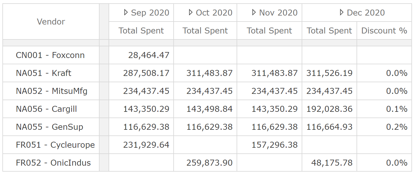
In order to introduce our second hierarchy-grouping topic, let's take the following table as our requirement.
 |
What is interesting about this example is that the Dec 2020 member is combined with two measures, whilst all preceding months are combined with only one member. This would appear to break the different-hierarchy sets are combined in that the Date.Calendar YQMD-hierarchy members have not been combined with all measures.
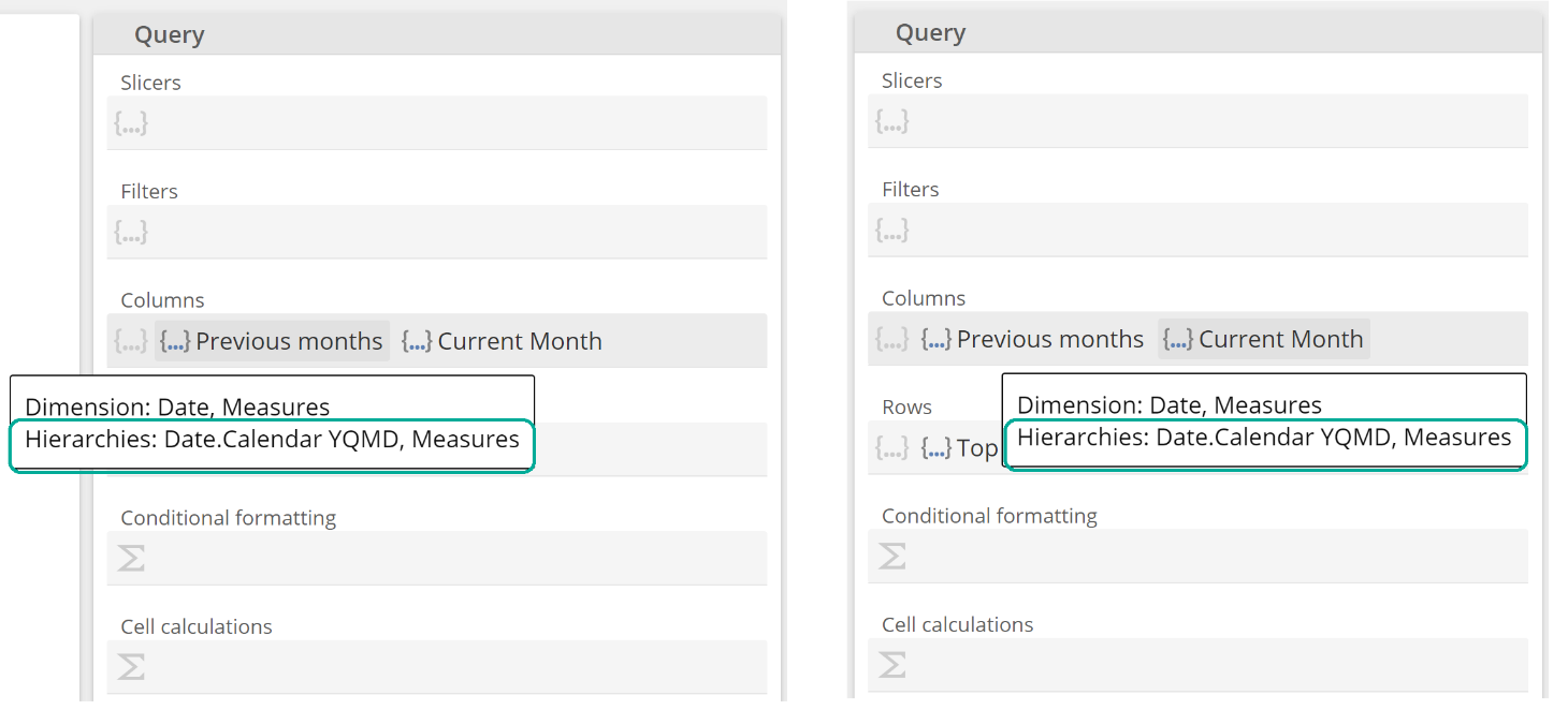
We won't step through building this particular example but instead, let's jump straight to how this table was designed and see why it's not a violation of our rule. From the following images, observe that the Columns placeholder holds two set tabs, and if we hover over each of the tabs, we can see that both provide Date.Calendar YQMD andMeasure hierarchy members/measures.
 |
Because the Previous months tab and the Current Month tab are both same-hierarchy, their results are appended. We can quickly look at the definition of each set to ensure this behavior is clear.
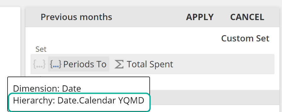
The Previous months tab is defined as follows. Note that it makes use of Periods To in order to return the previous three months, and it combines these three months with a calculated Total Spent measure.
 |
The result is that Previous months is now a set of combined Date.Calendar YQMD-hierarchy members and measures.
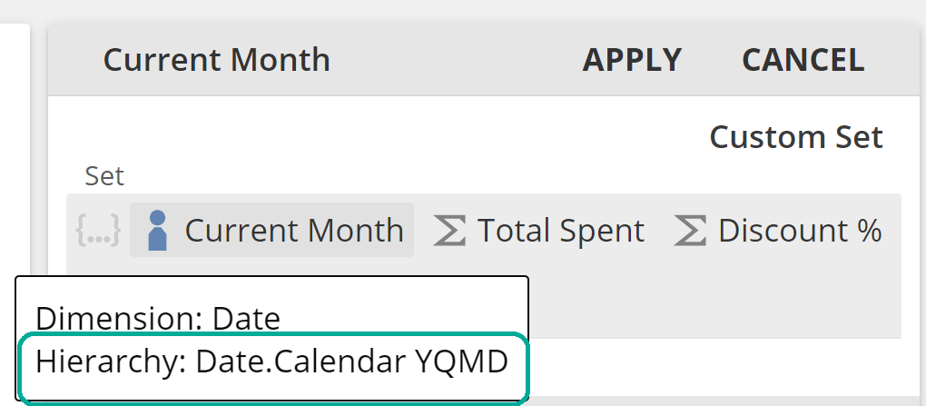
The Current month tab is defined as follows. In this case, we make of the Current Month Function and it with two calculated measures.
 |
The result is that the Current month set is also a set of combined Date.Calendar YQMD-hierarchy members and measures. With the definitions of the Previous months and Current month sets in mind, it is now possible to see how these two come together in the table headers.
 |
This example is a little different from all other Set Function examples to this point. The reason being, our sets were sets of member-measure combinations. You may also encounter a requirement for a set of member combinations, for example, a set of region-product combinations. Both of these scenarios are examples of multi-hierarchy sets. Should you meet these requirements, keep in mind the same hierarchy-grouping rules apply.
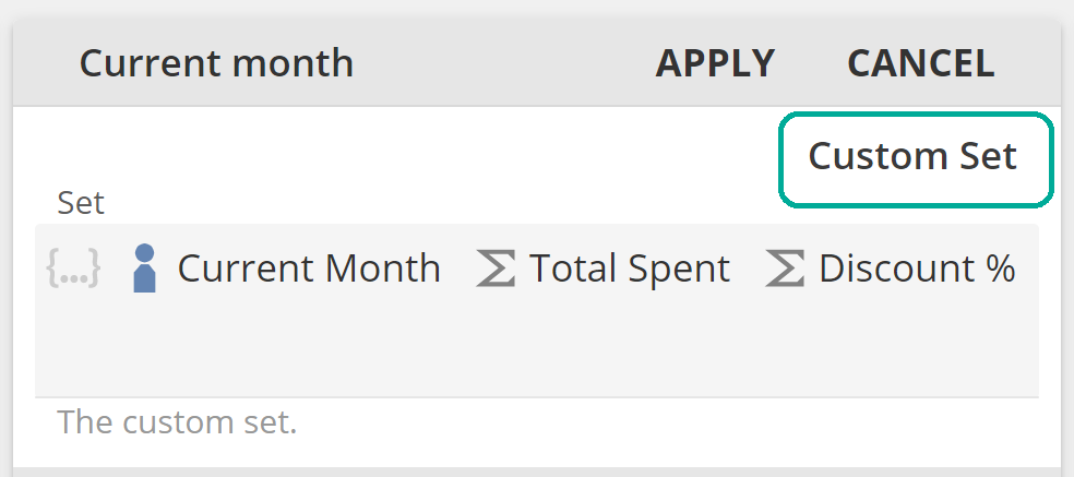
Just one final point on the example we just walked through. You may have noticed we made use of the Custom Set Function (keeping in mind Current month was only the title we provided).
 |
The Custom Set Function is only ever required when working with a multi-hierarchy set, as was the case above example. It is, however, still useful when working with a single hierarchy to improve the readability of a placeholder. We'll leave this for the reader to discover examples of this in their analytic journeying.
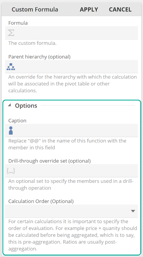
Additional function options
We are very close to the end of our discussion of Functions; however, we need to expand upon the Options section that you will have seen in our discussion on dynamic captions. Let’s use the Custom Formula for our discussion because it includes an additional Options field that isn’t available for all Functions. The Options section is expanded in the following.
 |
We’ll jump straight to the Drill-through override set, but before talking to its use, it’s important to understand that in most cases, the application is able to unambiguously determine the correct rows to show for a drill-through. The total of these rows should also add to the formula at hand. However, it is not always possible to satisfy these requirements. The Drill-through override set placeholder allows the designer to accommodate formulas for which the application cannot unambiguously determine the correct row set or for which the total of the rows won’t add to the formula.
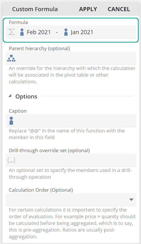
Let’s clarify this with an example. In the following image, the Formula placeholder is now populated, and we’d like to be able to drill through from the resulting cells to see the transaction records that make up our data.
 |
The challenge with this particular formula is that the application cannot unambiguously determine which records to show. Obviously, there will be no records transacted in Jan 2021 and Feb 2021. We might argue that this formula's focus is Feb 2021’s growth compared to Jan 2021, and as such, we should only show the records for Jan/Feb 2021. However, we could also argue that the formula uses records from both Jan 2021 and Feb 2021, so it should show records from both periods. In this case, we can be confident the rows won’t total to give the same value as the formula. The point being, there is ambiguity.
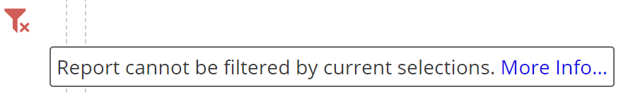
In the scenarios where the user attempts to drill through, and the application cannot unambiguously determine the transaction rows or the total cannot be matched, the following error will show.
 |
A similar scenario may occur when we configure a dashboard for inter-cell slicing (we will see how to configure this in the Dashboards section). In such a case, the following error will show.
 |
In both cases, the More info link provides guidance on the specific aspect of the formula that is introducing ambiguity. For example, in the case above, the non-additional operator is the root of the issue.
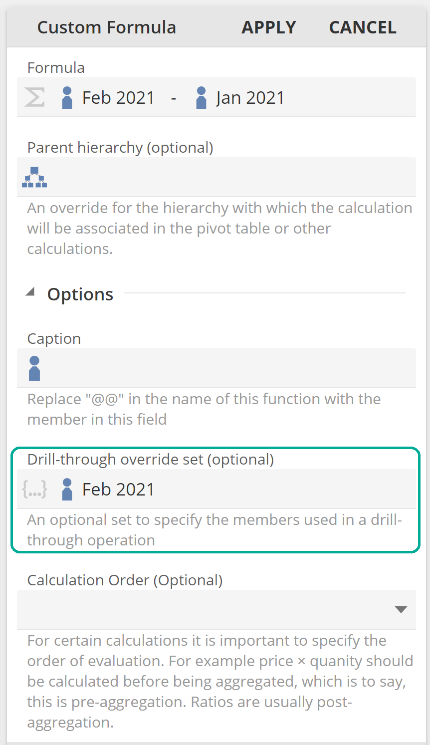
Let’s assume the designer has decided that drill-through should provide only the Feb 2021 records on the basis that the focus of the formula Feb 2021’s growth compared to Jan 2021. This is a simple matter of dragging the Feb 2021 member from the Dimension tree to the Drillthrough override set placeholder, as in the following image.
 |
For more information on populating the Drillthrough override set placeholder, see the Drillthrough override sets section from the Analytic functions article.
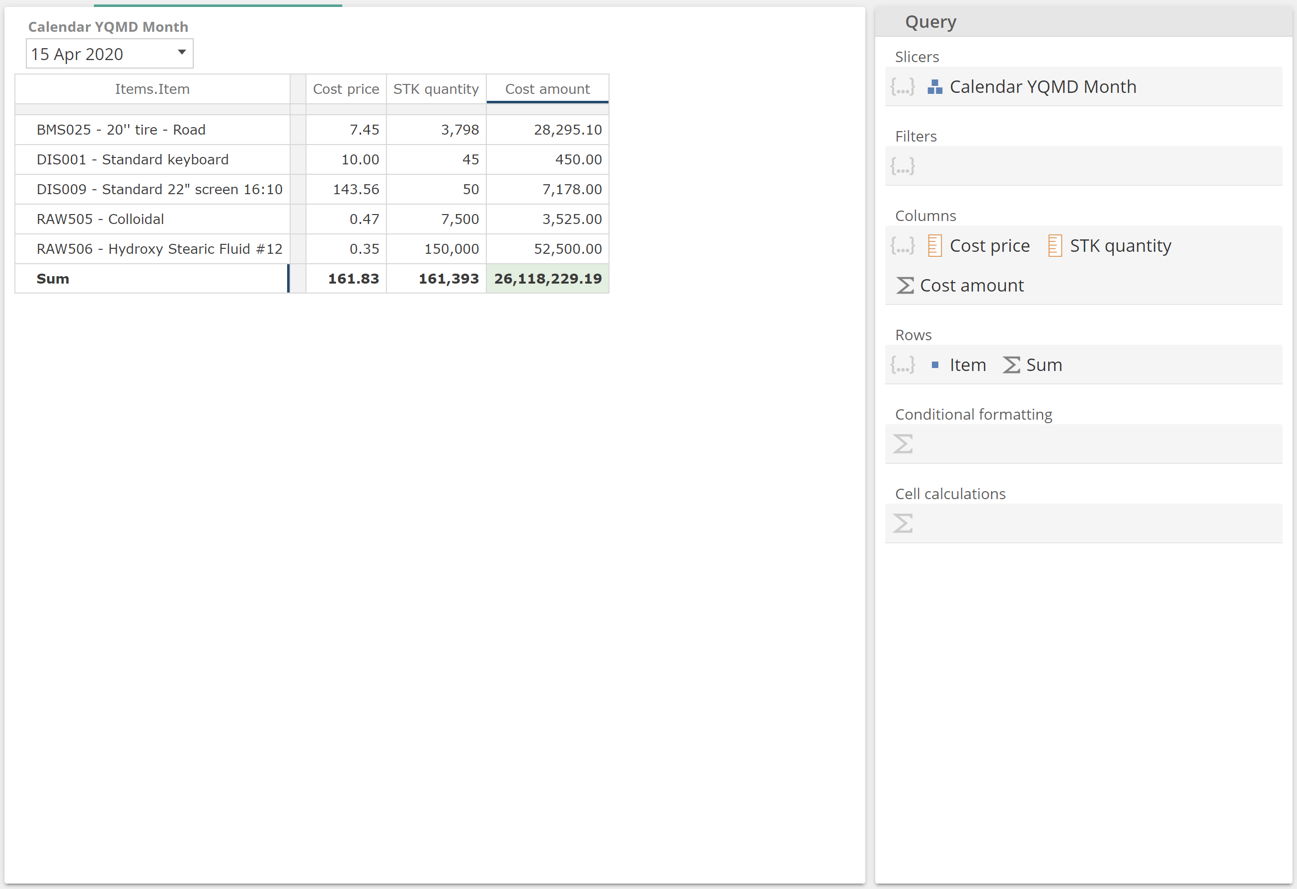
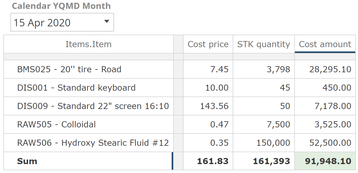
Turning now to Calculation Order. Because Analysis Reports allow for formulas on both Rows and Columns (or their chart equivalents), the analytic designer needs to be conscious of implications where these formulas intersect. Let’s start with our example.
 |
In the above image, we have two formulas Cost amount(defined as Cost price x STK quantity) and Sum (of the Item level). Everything is rosy, except for the cell where these two formulas intersect. It should be relatively obvious that the Cost amount column does not sum to the bottom-right cell. Instead, the value we are seeing is the product of the sum-of-costs and the sum-of-quantities (161.83 x 161,393).
Let’s quickly define aggregation(also summarization) as a means of combing many numbers into one. By this definition, summing, averaging, taking the minimum, and taking the maximum are all forms of aggregation. Returning to our example, we can now say that the bottom right formula is the result of:
Aggregating (summing in this case) the item prices.
Aggregating (summing in this case) the item quantities.
Taking the product of these sums.
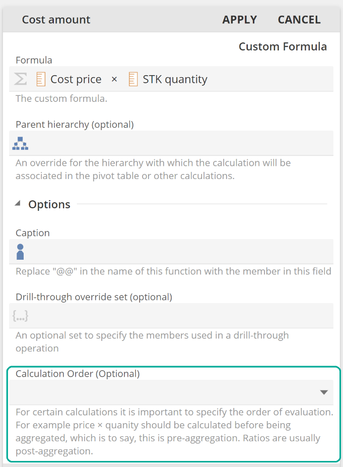
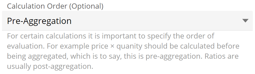
Stating it in this way, we might say the bottom-right cell Cost amount formula has been evaluated post-aggregation. And from this, we can see that in order to correct the formula, we want to ensure it is evaluated pre-aggregation. Again, to be clear, it is the Cost amount formula that should be evaluated pre-aggregation, so we turn we must set the Cost amount'sCalculation Order.
 |
From the drop-down select Pre-Aggregation.
 |
Click Apply, and things are now as they should be.
 |
This time we can say that the bottom right formula is the result of:
Taking the product of item prices and item quantities
Aggregating (summing in this case) these products
The Cost amount formula has been evaluated pre-aggregation, exactly as specified.
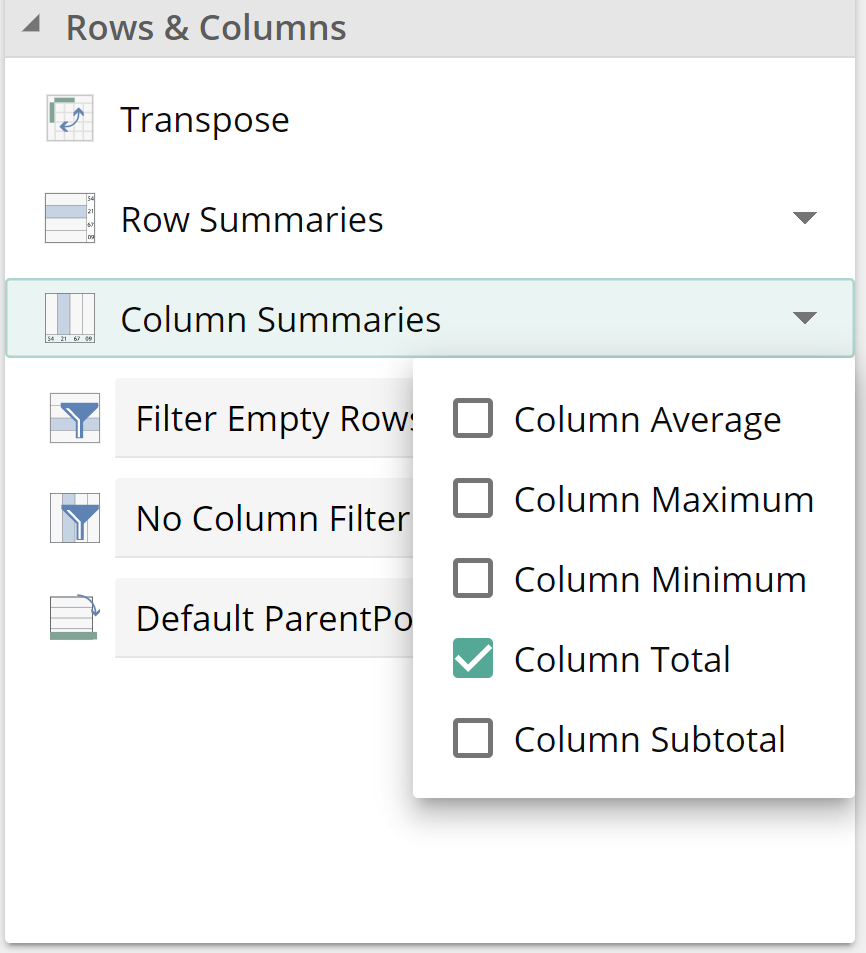
This example made use of the Sum function to provide a column total. Importantly the table's built-in Summaries are also formulas and may result in formula intersections. If we remove the Sum Function (right-click Remove from the placeholder tab menu), we can get the same result by applying Column Total.
 |
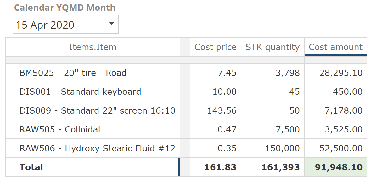
And by merit of the Cost amount calculation being pre-aggregation, the Cost amount total (bottom right) continues to provide the correct value.
 |
Fortunately, the scenarios where Calculation Order affects the value of an intersecting cell are relatively rare for the following two reasons:
It is not necessary to consider Calculation Order if both formulas use only + and – or summation functions (those with “total” or “sum” in their title).
Most analytic require post-aggregation, which is the default.
Furthermore, as from the example at hand, scenarios where Calculation Order requires configuration usually result in identifiably wrong numbers. For additional examples and further discussion of Calculation Order, see the Calculation Order section from the Analytic Functions article.
And that’s Functions! It’s been a lot to discuss, and for this reason, do consider rereading this section again in the future. Functions are key to the flexible analytics that Data Hub provides. From here, we can move to some relatively simpler topics.
Calculated Member & Named Sets
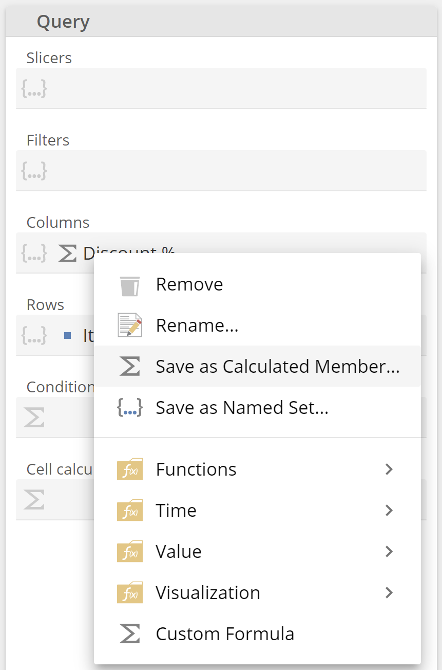
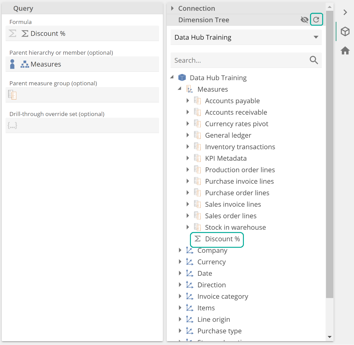
It is common to find a formula that you wish to use across multiple analytics. For example, let's take the Discount %we defined previously. If you right-click, the placeholder tab menu will show and provide the option to Save as Calculated Member, as in the following image.
 |
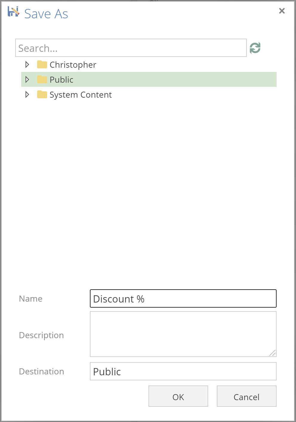
And now we see that a Calculated Member is itself a resource of the application, and we must decide where to save it.
|
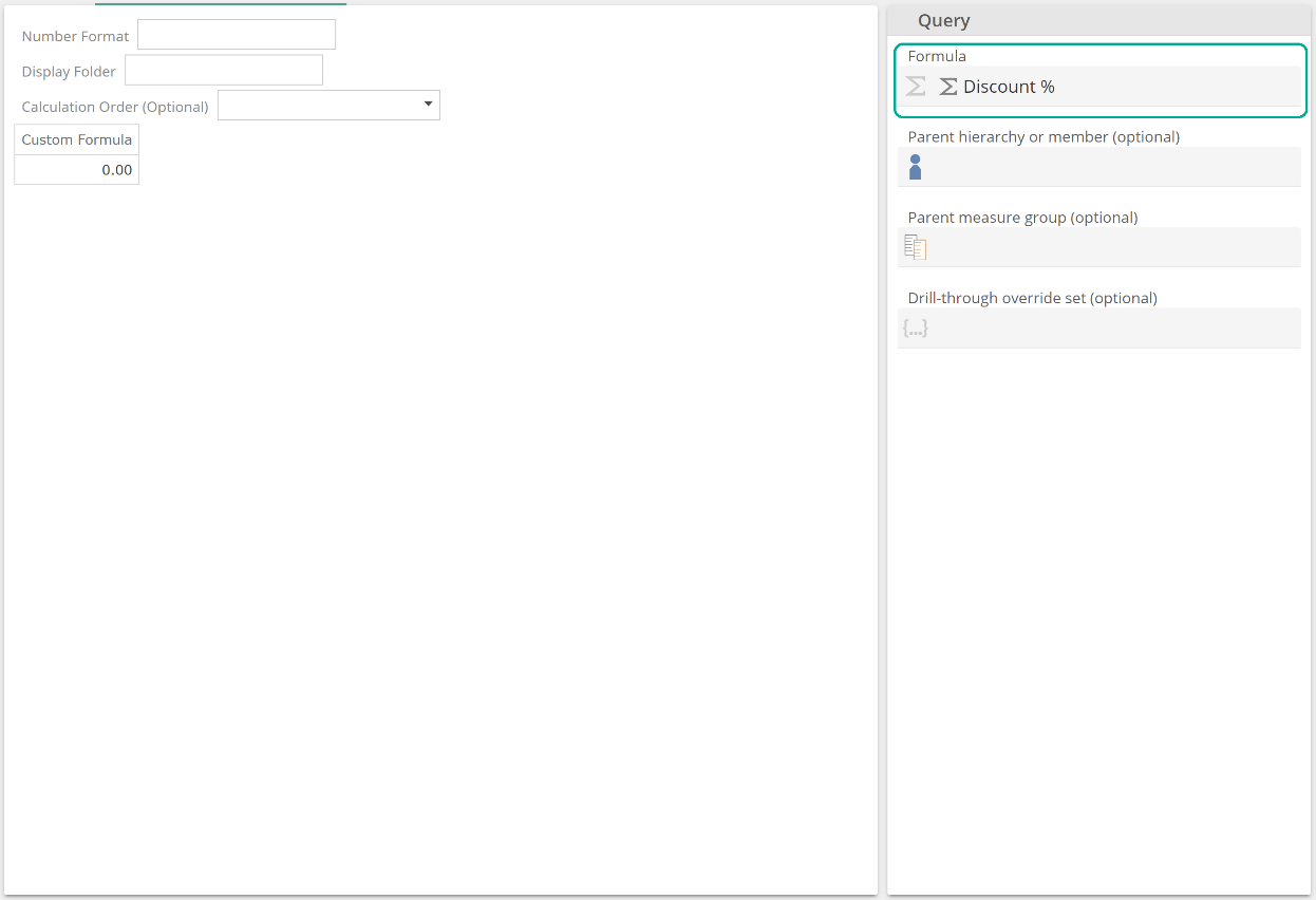
The new Calculated Member's design now shows with the Formula placeholder's wrapped Function.
 |
It is also possible to get to create a Calculated Member from the New resource button; however, the approach provided above is generally more useful because you can design the formula in the context of an Analysis Report.
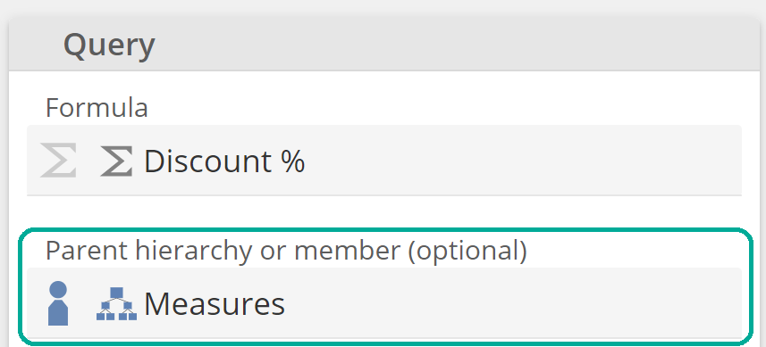
There are two ways to use a Calculated Member resource. You can drag it from the Resource Explorer into the relevant query placeholder. Alternatively, if you specify a Group-by hierarchy or parent member, you will find a newly-created Calculated Member on the Dimension Tree. In this case, given we would like to treat Discount % as a measure (and group it with other measures), drag Measures from the Dimension Tree to populate the Group-by hierarchy or parent member placeholder, as in the following.
 |
If you save at this point and click Refresh on the Dimension Tree, you will be able to see our new Calculated Member (or we may call it a Calculated Measure in this case).
 |
We’ll leave moving this calculation to a measure group folder as an exercise for the reader. And we’ll leave the discussion of the additional Calculated Member design fields to the online documentation’s Calculated Members article.
Before moving on, some guidance on analytic design, you may notice that the pre-built analytics make use of many simple Calculated Members that don’t otherwise appear to be justified. Whilst simple, these Calculated Members serve as the single-source-of-truth for this formula's definition. For example, there are many calculations used by the pre-built financial statements whose formula is a single member. However, should this single-member require changing, this design pattern ensures it is only changed in one place. It is worth keeping this pattern in mind as you build out your analytics and particularly any complex analytics.
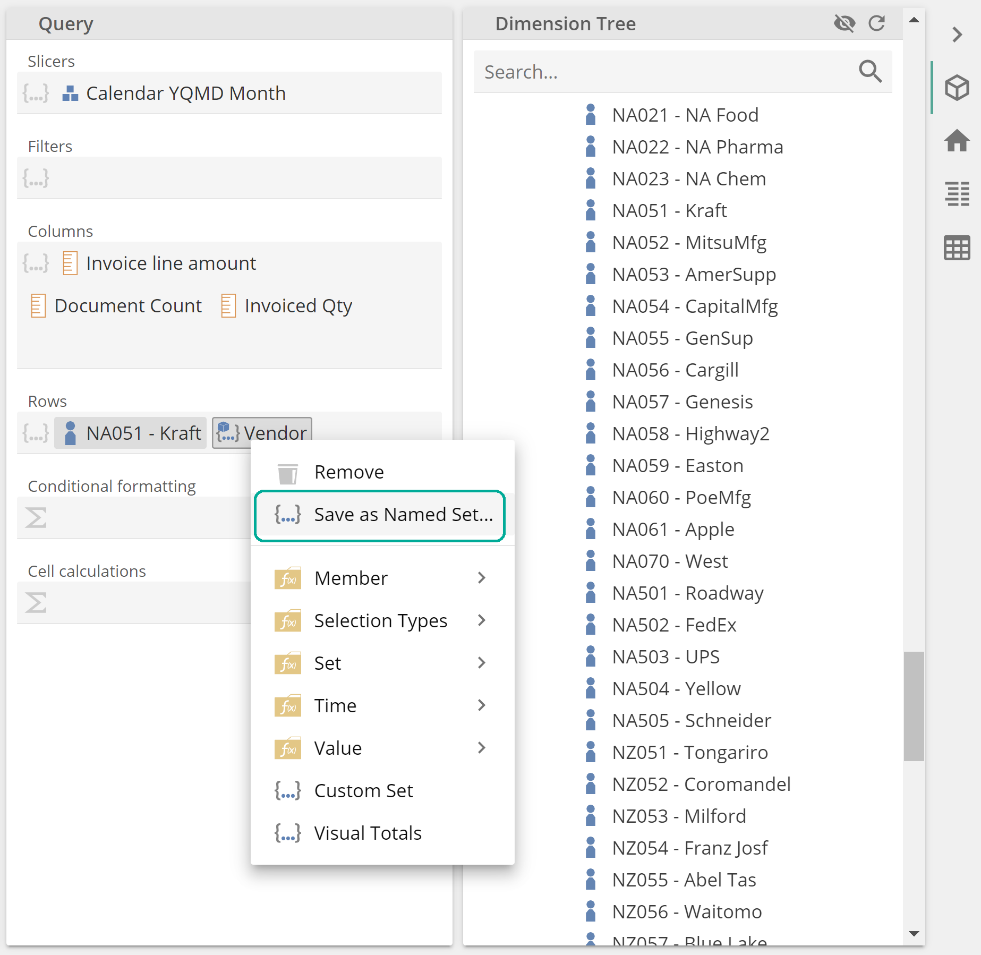
Named Sets work similarly to Calculated Members. To show the Save as Named Setoption in the placeholder tab menu, ensure a set tab is selected or ensure multiple items are selected (using Ctrl-click and Shift-click). From an earlier example, we’ve Shift-clicked to select both the NA051 and Vendor tabs in the following image.
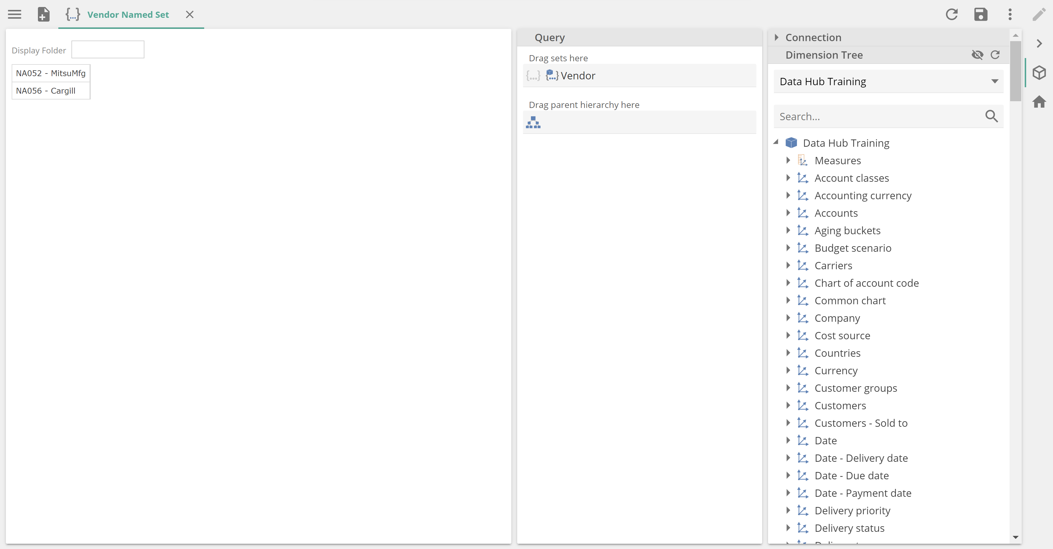 |
Clicking on Save as Named Set will show a pop-up prompting for a save location before you are taken to the Named Set design, as in the following.
 |
As with Calculated Members, a Named Set may be used from the Resource Explorer or the Dimension Tree, where the Parent hierarchy placeholder has been populated.